

pandas is a software library written in Python and is the basis for data manipulation and analysis in the language. Its name comes from "panel data," an econometrics term for datasets that include observations over multiple time periods for the same individuals.
pandas offers a collection of high-performance, easy-to-use, and intuitive data structures and analysis tools that are of great use to marketing analysts and data scientists alike. It has the following two primary object types:
DataFrame: This is the fundamental tabular relationship object that stores data in rows and columns (like a spreadsheet). To perform data analysis, functions and operations can be directly applied to DataFrames.
Series: This refers to a single column of the DataFrame. The value can be accessed through its index. As Series automatically infers a type, it automatically makes all DataFrames well-structured.
The following figure illustrates a pandas DataFrame with an automatic integer index (0, 1, 2, 3...):
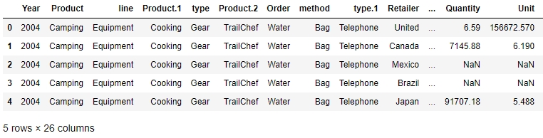
Figure 1.4: A sample pandas DataFrame
Now that we understand what pandas objects are and how they can be used to automatically get structured data, let's take a look at some of the functions we can use to import and export data in pandas and see if the data we passed is ready to be used for further analyses.
Every team in a marketing group can have its own preferred data type for their specific use case. Those who have to deal with a lot more text than numbers might prefer using JSON or XML, while others may prefer CSV, XLS, or even Python objects. pandas has a lot of simple APIs (application program interfaces) that allow it to read a large variety of data directly into DataFrames. Some of the main ones are shown here:
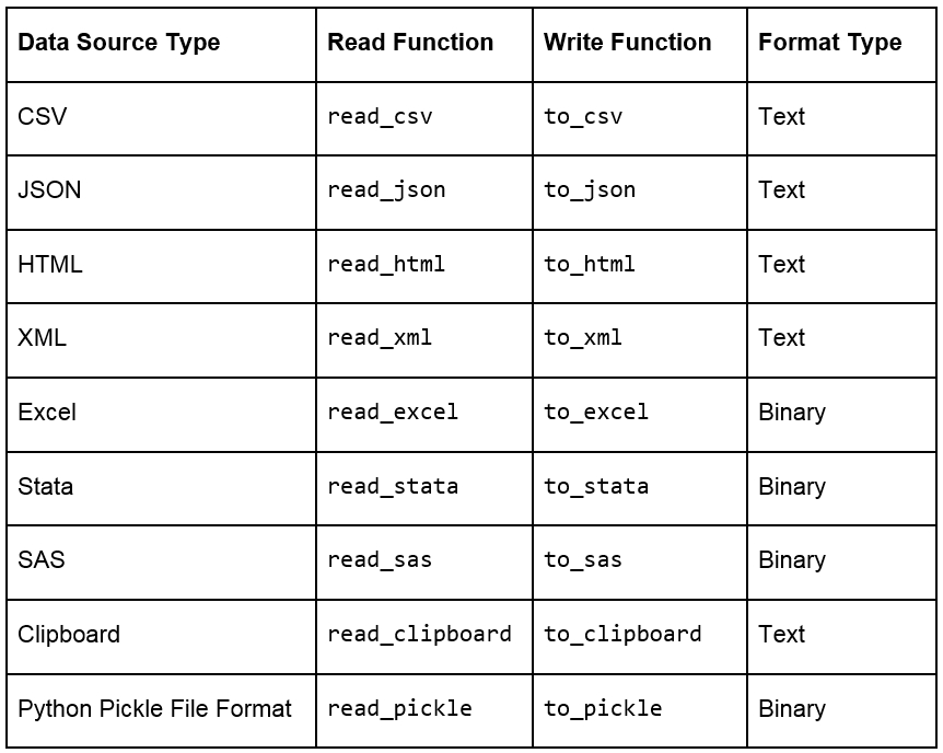
Figure 1.5: Ways to import and export different types of data with pandas DataFrames
Note
Remember that a well-structured DataFrame does not have hierarchical or nested data. The read_xml, read_json(), and read_html() functions (and others) cause the data to lose its hierarchical datatypes/nested structure and convert it into flattened objects such as lists and lists of lists. Pandas, however, does support hierarchical data for data analysis. You can save and load such data by pickling from your session and maintaining the hierarchy in such cases. When working with data pipelines, it's advised to split nested data into separate streams to maintain the structure.
When loading data, pandas provides us with additional parameters that we can pass to read functions, so that we can load the data differently. Some additional parameters that are used commonly when importing data into pandas are given here:
skiprows = k: This skips the first k rows.
nrows = k: This parses only the first k rows.
names = [col1, col2...]: This lists the column names to be used in the parsed DataFrame.
header = k: This applies the column names corresponding to the kth row as the header for the DataFrame. k can also be None.
index_col = col: This sets col as the index of the DataFrame being used. This can also be a list of column names (used to create a MultiIndex) or None.
usecols = [l1, l2...]: This provides either integer positional indices in the document columns or strings that correspond to column names in the DataFrame to be read. For example, [0, 1, 2] or ['foo', 'bar', 'baz'].
Once you've read the DataFrame using the API, as explained earlier, you'll notice that, unless there is something grossly wrong with the data, the API generally never fails, and we always get a DataFrame object after the call. However, we need to inspect the data ourselves to check whether the right attribute has received the right data, for which we can use several in-built functions that pandas provides. Assume that we have stored the DataFrame in a variable called df then:
df.head(n) will return the first n rows of the DataFrame. If no n is passed, by default, the function considers n to be 5.
df.tail(n) will return the last n rows of the DataFrame. If no n is passed, by default, the function considers n to be 5.
df.shape will return a tuple of the type (number of rows, number of columns).
df.dtypes will return the type of data in each column of the pandas DataFrame (such as float, char, and so on).
df.info() will summarize the DataFrame and print its size, type of values, and the count of non-null values.
For this exercise, you need to use the user_info.json file provided to you in the Lesson01 folder. The file contains some anonymous personal user information collected from six customers through a web-based form in JSON format. You need to open a Jupyter Notebook, import the JSON file into the console as a pandas DataFrame, and see whether it has loaded correctly, with the right values being passed to the right attribute.
Note
All the exercises and activities in this chapter can be done in both the Jupyter Notebook and Python shell. While we can do them in the shell for now, it is highly recommended to use the Jupyter Notebook. To learn how to install Jupyter and set up the Jupyter Notebook, check https://jupyter.readthedocs.io/en/latest/install.html. It will be assumed that you are using a Jupyter Notebook from the next chapter onward.
Note
The 64 displayed with the type above is an indicator of precision and varies on different platforms.
Open a Jupyter Notebook to implement this exercise. Once you are in the console, import the pandas library using the import command, as follows:
import pandas as pd
Read the user_info.json JSON file into the user_info DataFrame:
user_info = pd.read_json("user_info.json")Check the first few values in the DataFrame using the head command:
user_info.head()
You should see the following output:
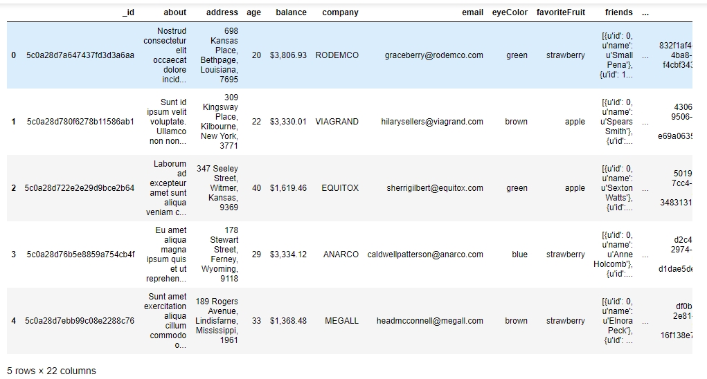
Figure 1.6: Viewing the first few rows of user_info.json
As we can see, the data makes sense superficially. Let's see if the data types match too. Type in the following command:
user_info.info()
You should get the following output:
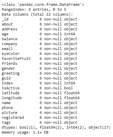
Figure 1.7: Information about the data in user_info
From the preceding figure, notice that the isActive column is Boolean, the age and index columns are integers, whereas the latitude and longitude columns are floats. The rest of the elements are Python objects, most likely to be strings. Looking at the names, they match our intuition. So, the data types seem to match. Also, the number of observations seems to be the same for all fields, which implies that there has been no data loss.
Let's also see the number of rows and columns in the DataFrame using the shape attribute of the DataFrame:
user_info.shape
This will give you (6, 22) as the output, indicating that the DataFrame created by the JSON has 6 rows and 22 columns.
Congratulations! You have loaded the data correctly, with the right attributes corresponding to the right columns and with no missing values. Since the data was already structured, it is now ready to be put into the pipeline to be used for further analysis.
In this exercise, you will be using the data.csv and sales.xlsx files provided to you in the Lesson01 folder. The data.csv file contains the views and likes of 100 different posts on Facebook in a marketing campaign, and sales.xlsx contains some historical sales data recorded in MS Excel about different customer purchases in stores in the past few years. We want to read the files into pandas DataFrames and check whether the output is ready to be added into the analytics pipeline. Let's first work with the data.csv file:
Import pandas into the console, as follows:
import pandas as pd
Use the read_csv method to read the data.csv CSV file into a campaign_data DataFrame:
campaign_data = pd.read_csv("data.csv")Look at the current state of the DataFrame using the head function:
campaign_data.head()
Your output should look as follows:
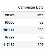
Figure 1.8: Viewing raw campaign_data
From the preceding output, we can observe that the first column has an issue; we want to have "views" and "likes" as the column names and for the DataFrame to have numeric values.
We will read the data into campaign_data again, but this time making sure that we use the first row to get the column names using the header parameter, as follows:
campaign_data = pd.read_csv("data.csv", header = 1)Let's now view campaign_data again, and see whether the attributes are okay now:
campaign_data.head()
Your DataFrame should now appear as follows:
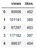
Figure 1.9: campaign_data after being read with the header parameter
The values seem to make sense—with the views being far more than the likes—when we look at the first few rows, but because of some misalignment or missing values, the last few rows might be different. So, let's have a look at it:
campaign_data.tail()
You will get the following output:
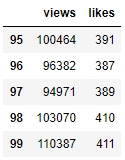
Figure 1.10: The last few rows of campaign_data
There doesn't seem to be any misalignment of data or missing values at the end. However, although we have seen the last few rows, we still can't be sure that all values in the middle (hidden) part of the DataFrame are okay too. We can check the datatypes of the DataFrame to be sure:
campaign_data.info()
You should get the following output:
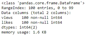
Figure 1.11: info() of campaign_data
We also need to ensure that we have not lost some observations because of our cleaning. We use the shape function for that:
campaign_data.shape
You will get an output of (100, 2), indicating that we still have 100 observations with 2 columns. The dataset is now completely structured and can easily be a part of any further analysis or pipeline.
Let's now analyze the sales.xlsx file. Use the read_excel function to read the file in a DataFrame called sales:
sales = pd.read_excel("sales.xlsx")Look at the first few rows of the sales DataFrame:
sales.head()
Your output should look as follows:

Figure 1.12: First few rows of sales.xlsx
From the preceding figure, the Year column appears to have matched to the right values, but the line column does not seem to make much sense. The Product.1, Product.2, columns imply that there are multiple columns with the same name! Even the values of the Order and method columns being Water and Bag, respectively, make us feel as though something is wrong.
Let's look at gathering some more information, such as null values and the data types of the columns, and see if we can make more sense of the data:
sales.info()
Your output will look as follows:
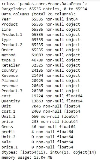
Figure 1.13: Output of sales.info()
As there are some columns with no non-null values, the column names seem to have broken up incorrectly. This is probably why the output of info showed a column such as revenue as having an arbitrary data type such as object (usually used to refer to columns containing strings). It makes sense if the actual column names start with a capital letter and the remaining columns are created as a result of data spilling from the preceding columns.
Let's try to read the file with just the new, correct column names and see whether we get anything. Use the following code:
sales = pd.read_excel("sales.xlsx", names = ["Year", "Product line", "Product type", "Product", "Order method type", "Retailer Country", "Revenue", "Planned revenue", "Product cost", "Quantity", "Unit cost", "Unit price", "Gross Profit", "Unit sale price"])You get the following output:
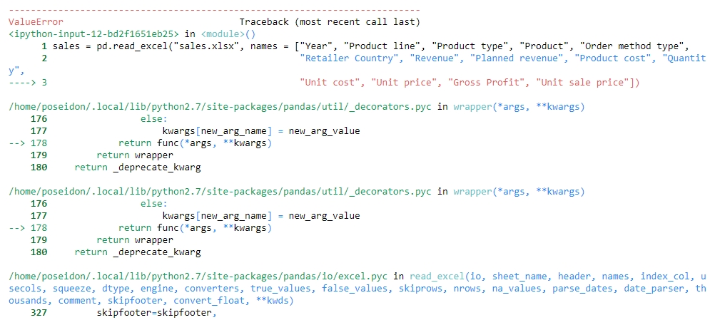
Figure 1.14: Attempting to structure sales.xlsx
Unfortunately, the issue is not just with the columns, but with the underlying values too. The value of one column is leaking into another and thus ruining the structure. Understandably, the code fails because of length mismatch. Therefore, we can conclude that the sales.xlsx data is very unstructured.
With the use of the API and what we know up till this point, we can't directly get this data to be structured. To understand how to approach structuring this kind of data, we need to dive deep into the internal structure of pandas objects and understand how data is actually stored in pandas, which we will do in the following sections. We will come back to preparing this data for further analysis in a later section.
Let's say you want to store some values from a data store in a data structure. It is not necessary for every element of the data to have values, so your structure should be able to handle that. It is also a very common scenario where there is some discrepancy between two data sources on how to identify a data point. So, instead of using default numerical indices (such as 0-100) or user-given names to access it, like in a dictionary, you would like to access every value by a name that comes from within the data source. This is achieved in pandas using a pandas Series.
A pandas Series is nothing but an indexed NumPy array. To make a pandas Series, all you need to do is create an array and give it an index. If you create a Series without an index, it will create a default numeric index that starts from 0 and goes on for the length of the Series, as shown in the following figure:
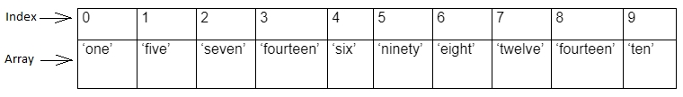
Figure 1.15: Sample pandas Series
Note
As a Series is still a NumPy array, all functions that work on a NumPy array, work the same way on a pandas Series too.
Once you've created a number of Series, you might want to access the values associated with some specific indices all at once to perform an operation. This is just aggregating the Series with a specific value of the index. It is here that pandas DataFrames come into the picture. A pandas DataFrame is just a dictionary with the column names as keys and values as different pandas Series, joined together by the index:
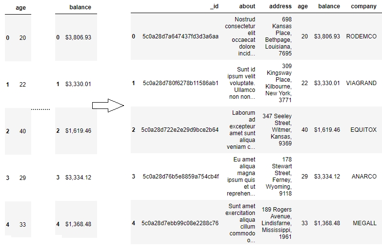
Figure 1.16: Series joined together by the same index create a pandas Dataframe
This way of storing data makes it very easy to perform the operations we need on the data we want. We can easily choose the Series we want to modify by picking a column and directly slicing off indices based on the value in that column. We can also group indices with similar values in one column together and see how the values change in other columns.
Other than this one-dimensional Series structure to access the DataFrame, pandas also has the concept of axes, where an operation can be applied to both rows (or indices) and columns. You can choose which one to apply it to by specifying the axis, 0 referring to rows and 1 referring to columns, thereby making it very easy to access the underlying headers and the values associated with them:
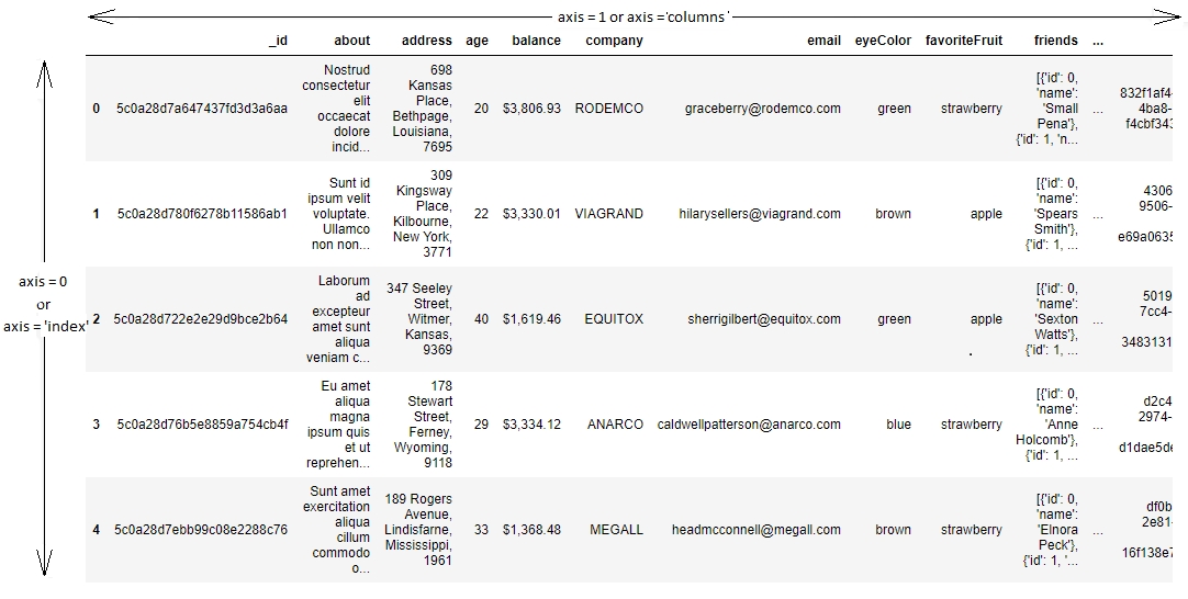
Figure 1.17: Understanding axis = 0 and axis = 1 in pandas