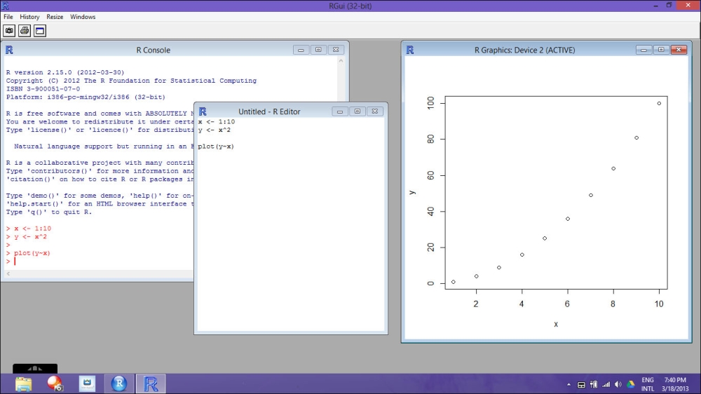
As soon as you start R, you will see that a workspace is open; you can see a screenshot of the R Console window in the following image. The workspace is the environment in which you are working; where you will load your data and create your variables. As soon as you close R, the program will ask you if you want to save the workspace on the hard drive of the computer. Loading a previously saved workspace will allow you to find again all the objects that you have created in the previous session.

You can save the workspace in the cascade menu by navigating to File | Save Workspace…. Alternatively, you can also save the workspace with the command save.image(). This will create a file called .RData in your working directory. The working directory is basically the location on your computer where R is operating. This means that in such a directory, R is able to read and write files. You can identify which is your working directory with the help of the command getwd(). You may change your working directory with the command setwd("dir"), where "dir" is the directory address. While this last option may be very useful within script files, in a more common situation it will be easier to change the working directory via the GUI by navigating to File | Change dir….

Now that you have already typed some commands in the R shell, you will probably have already noticed a couple of things. R is case sensitive; this means that if you type Setwd() instead of setwd(), you will get an error. You will also have probably noticed that most of the commands you saw end with a couple of parentheses. The parentheses indicate that what you are using is not an object, but a function. Within the parentheses, you may specify the arguments of the function (an example is the function library() that you have already encountered previously), while if the function doesn't need any argument or if you intend to use only default values, you don't need any argument within the parentheses. We will go more in detail on this matter in the section Top features you'll want to know about. Finally you also noticed that typing your command directly in the R shell is not really optimal. One efficient way of interacting with the shell is via scripts. In this method, you can write your code in a separate window and then you can execute the code in the shell, so that if you would need to save your code or execute it several times you will not have to type it again. You can do that also in the basic R interface by navigating to File | New script. Once you have some commands in the script window, you will need to execute them in the console. Of course you can do copy-paste as usual, but it is better to select with your mouse the code you intend to execute and press the keys Ctrl + R. Alternatively, you can also right-click in the window and select Run line or selection.

These are some additional functions that you can use to keep an eye on your workspace. Let's create a variable, x, with a numeric value using the following code:

> x <- 10

If you would like to know which variables you have created in the current session, you can use the command objects() or ls(), while if you would like to see which libraries and data frames are attached in the workspace, you can use the command search(). R keeps a record of all the commands you type. For example, to save the history in a file named myHistory, use the savehistory(file = "myHistory") command, and to load the history file named myHistory, use loadhistory(file = "myHistory"). If you save your workspace image when quitting, then your current history will be saved in .Rhistory in the current working directory.

The screen prompt, >, is the R prompt that waits for commands. In this book, all the R code that is typed in this prompt will be preceded by the symbol >. The [1] that prefixes the output indicates that this is item one in a vector of output, and will be reported together with the output results to make them easier to be identified. All the functions will be followed by double brackets in the text.

On the start-up screen, you can either type any function, command, or you can use R to perform basic calculations. R uses the usual symbols for addition (+), subtraction (-), multiplication (*), division (/), and exponentiation (^). Parentheses ( ) can be used to specify the order of operations. R also provides %% for taking the modulus and %/% for integer division. Comments in R are defined by the character #; so everything after such characters up to the end of the line will be ignored by R.

R has a number of built-in functions, such as sin(x), cos(x), tan(x), (all in radians), exp(x), log(x), and sqrt(x). Some special constants such as pi are also predefined. You can see an example of the use of such a function in the following code:

> exp(2.5)
[1] 12.18249

You can write a command on each line, or you can divide longer lines of commands in more than one line if the line is incomplete according to the R language (for example, with a comma, an operator, or with more left parentheses than right parentheses, implying that more right parentheses will follow). When the submitted line is not complete, the R prompt changes from > to +. For example, you can divide a sum on two lines by pressing Enter after each number:

> 5+
+ 5
[1] 10

If you have made a mistake and you want to get rid of the + prompt and return to the > prompt, either press the Esc key or the Stop button in the GUI.

As you already have probably noticed, in R, a certain value is assigned to an object by assignment. This is achieved by the arrow operator <-, which is a composite symbol made up of the less than sign and minus sign with no space between them. Thus, to create a scalar constant x with a value 5, we type:

> x<-5

The command x=5 also works in R, but the arrow option is usually preferred. The direction of the arrow represents the direction of the assignment; so x<-5 and 5->x have the same result. Be aware that there is a potential ambiguity if you get the spacing wrong. In fact, comparing the assignment x<-5, "x gets 5", with x < -5 becomes a logical question, which is asking if x is less than minus 5, and will produce an answer TRUE or FALSE.

At this point, you have obtained an idea of the way R works, and you have already learned how you can specify the arguments within a function. Many things in R are done via function calls. The format of such calls is the name of the function followed by a parenthesis containing the arguments separated by a comma. The arguments passed to the function may be assigned directly within the body of the function or they can be defined in the workspace and then recalled within the function.

One example of a function with multiple arguments is the function rnorm. Such a function requires the arguments rnorm(n, mean, sd) and can be used to simulate n values from a distribution with mean and standard deviation provided within the function. You could provide such arguments in two different ways:

> rnorm(n=10, mean=0, sd=1)

or

> rnorm(10, 0, 1)

In the second way, since the values are not associated with a specific argument, R will assume that they will be provided in an order, first n, then mean, and finally sd. This is known as positional matching. Also, keep in mind that if the function does not require any argument, you will still need to include the parenthesis after the function name. By executing only the name of the function (without brackets), you will have access to the actual code, which is defined in the function itself. This may be helpful in some cases if you would like to know what exactly a function does.

Many packages, external or included in the basic R distribution, come with built-in datasets. In some cases the data is already available in the R workspace directly, while in some other situations it requires a specific call to the data function with the name of the dataset to load as an argument. Particularly at the beginning of your learning experience (but also once you become more experienced), it may be very handy to have access to the same data, particularly if you would like to do some tests with the function that you are just learning. You can access the list of the available datasets with a short description of the data by just using the command data().

In some cases, you may find out that the calculation you perform in R may lead to a special value: infinity. Such a value is represented in R by Inf or –Inf. You can easily see an example of that by dividing a number by zero:

> 17/0
[1] Inf

The value infinity, as you have seen, may be returned by R during a calculation, but it may also be provided as an argument within calculations:

> exp(-Inf)
[1] 0

Some other calculations may lead to results that are not numbers. Such quantities are defined in R as "Not a Number", and are represented by NaN. Some typical examples of such calculations are:

> 0/0
[1] NaN
> Inf/Inf
[1] NaN

A completely different situation is the one for which a certain value is not available, for example, in data collection. Such a missing value is represented by NA. You need to clearly understand the difference between NA and NaN, since they refer to different classes of values and they are treated differently in R. Missing values may be represented with the characters NA in the data, and in such a case, normally R will import them as NA values. In some cases, the values that are not identified, such as dots or blank spaces in the data sheet, may be read as NA values in R. Such values will be particularly important in statistical tests and data manipulation.

In R, there are a series of functions with the objective of testing objects for all these different classes of values. These are some examples of such functions:

> x <- Inf
> y <- NaN
> z <- NA
> is.infinite(x)
[1] TRUE
> is.nan(y)
[1] TRUE
> is.na(z)
[1] TRUE

A logical expression is formed using the comparison operators <, >, <=, >=, == (equal to), and != (not equal to), and the logical operators & (and), | (or), and ! (not). The order of operations can be controlled using parentheses ().

The value of a logical expression is either TRUE or FALSE. The integers 1 and 0 can also be used to represent TRUE and FALSE respectively (which is an example of what is called coercion). This is an easy example of a logical expression:

> c(1,2,3,4)==3
[1] FALSE FALSE TRUE FALSE

The previous example also shows how logical expressions can be applied to vectors, generating logical vectors of TRUE/FALSE values.

The basic object in R is the vector; even scalars are vectors of length 1. Vectors can be thought of as a series of data of the same class. There are six basic vector types (called atomic vectors): logical, integer, real, complex, string (or character), and raw. Integer and real represent numeric objects; logicals are Boolean data types with a possible value of TRUE or FALSE. Among such atomic vectors, the more common ones are logical, string, and numeric (integer and real).

There are several ways to create vectors.

The operator : (colon) is a sequence-generating operator; it creates sequences by incrementing or decrementing by one. The following are some examples:

> 1:10
 [1]  1  2  3  4  5  6  7  8  9 10
> 5:-6
 [1]  5  4  3  2  1  0 -1 -2 -3 -4 -5 -6

If the interval between the numbers is not 1, you can use the seq() function. Its arguments are the initial value of the series, the final one, and the increment. You can also generate a downward sequence if the increment is negative. If the increment does not match exactly the final value that you provided, the sequence will stop at the last matching number before the final value. Following are some examples:

> seq(from=2, to=2.5, by=0.1)
[1] 2.0 2.1 2.2 2.3 2.4 2.5
> seq(from=0, to=-2, by=-0.5)
[1]  0.0 -0.5 -1.0 -1.5 -2.0
> seq(from=1, to=2.7, by=0.5)
[1] 1.0 1.5 2.0 2.5

If the elements of your vector do not follow a specific series, or if they are not numeric, as alternative you may use the concatenation function c(). In such a function, you simply list the values of your vector separated by a comma. Here are some examples of numeric, logical, and character vectors. Remember that in R, character strings are defined by double-quotation marks.

> c(10,8,3,5,2)
> c(TRUE,FALSE,TRUE,TRUE)
> c("R","Programming")

One additional alternative in the creation of vectors is via the rep() function. Such a function will repeat a value (or a vector) n times. The vector to repeat and the number of repetitions are arguments to the function, which are provided to the function in the following order:

> rep(x=2, times=3)
[1] 2 2 2
> vec <-c(3,10,4)
> rep(x=vec, times=2)
[1]  3 10  4  3 10  4
> rep(x=vec, times=2, each=3)
 [1]  3  3  3 10 10 10  4  4  4  3  3  3 10 10 10  4  4  4

One of the more important features of R is the possibility to use an entire vector as arguments of functions, thus avoiding the use of cyclic loops. For example, the use of some of these functions is reported as follows, but remember that most of the functions in R also allow the use of vectors as arguments. In case you have any doubt about which kind of data is allowed for a specific argument in a function, remember to check the help page of that function.

> x <- c(12,10,4,6,9)
> max(x)
[1] 12
> min(x)
[1] 4
> mean(x)
[1] 8.2

Although we can apply functions directly to vectors, there are some cases in which you will need to access specific elements of the vector. This is possible in R via subscripts or indices. Indices allow identifying a specific element of an R object, and the same concept applies to a vector and also to a more complex data structure. In a vector, which is a one-dimensional object, they represent the position of the element in the vector, while if the object has two dimensions (for example, in a matrix), you will need to specify two positions (row number and column number). Indices must be specified within the [] operator, and in R, the element index starts from 1 and not from 0.

Remember, if a subscript appears as empty, it means that all the elements will be used; so when printing, the original vector remains unchanged while the negative index will exclude the element in that position. A couple of simple examples will make it clear how to use subscripts in vectors. Two-dimensional subscripts will be considered in the next sections.

> x <- c( 1,4,6,10)
> x[2]
[1] 4
> x[1:3]
[1] 1 4 6
> x[-2]
[1]  1  6 10

In R, the matrix notation is extended to elements of any kind, so it is possible to have a matrix of character strings. Matrices and arrays are basically vectors with a dimension attribute. You can see a very simple example of such an idea in the following code. The function dim() in the example returns a vector indicating the dimension of an object:

> x <- c("a","b","c","d")
> matrix(x,nrow=2)
     [,1] [,2]
[1,] "a"  "c" 
[2,] "b"  "d" 
> dim(x)
NULL
> y<- matrix(x,nrow=2)
> dim(y)
[1] 2 2

As you have seen in the example, the function matrix() may be used to create matrices. By default, such a function creates the matrix by column; as an alternative, it is possible to specify to the function to build the matrix by row:

> matrix(1:9,nrow=3,byrow=TRUE)
     [,1] [,2] [,3]
[1,]    1    2    3
[2,]    4    5    6
[3,]    7    8    9

Some useful functions when working with matrices are the functions to rename rows or columns—rownames() and colnames()—and the transposition function t(), which turns the rows into columns and columns into rows:

> x <- matrix(1:12,nrow=3)
> x
     [,1] [,2] [,3] [,4]
[1,]    1    4    7   10
[2,]    2    5    8   11
[3,]    3    6    9   12
> rownames(x) <- c("A","B","C")
> colnames(x) <- c("a","b","c","d")
> x
  a b c  d
A 1 4 7 10
B 2 5 8 11
C 3 6 9 12
> t(x)
   A  B  C
a  1  2  3
b  4  5  6
c  7  8  9
d 10 11 12

Remember that in a matrix, as well as in vectors, all elements must be of the same class; so it is not possible to have characters and numeric data together. In the following example, the first line of code produces a numeric matrix, while in the second one, since a character is provided in the matrix, R forces the other values to change to characters (that is why they appear between quotes).

> matrix(c(1,2,3,4),nrow=2)
     [,1] [,2]
[1,]    1    3
[2,]    2    4
> matrix(c(1,2,"c",4),nrow=2)
     [,1] [,2]
[1,] "1"  "c" 
[2,] "2"  "4"

Considering two matrices, x and y, other useful operations are matrix multiplication, x%*%y, transpose of a matrix, t(x), extracting the diagonal of a matrix, diag(x), inverse, solve(x), and determinant, det(x).

A list in R is a collection of different objects. One of the main advantages of lists is that the objects contained within a list may be of different types; for example, numeric and character values. In order to define a list, you simply will need to provide the object that you want to include as an argument of the function list():

> element1 <- c(1:9)
> element2 <- c("a","b","c")
> element3 <- matrix(1:9,nrow=3)
> list(element1, element2, element3)
[[1]]
[1] 1 2 3 4 5 6 7 8 9

[[2]]
[1] "a" "b" "c"

[[3]]
     [,1] [,2] [,3]
[1,]    1    4    7
[2,]    2    5    8
[3,]    3    6    9

As you can see, different elements may be combined together in one list object. Each of the listed objects is indicated with a double set of square brackets [[]]. You can use such an index to access an object, or as an alternative, you can rename the elements of the list. In the following example, you will notice how you can access a specific element using its name and the operator $:

> myList <- list(element1, element2, element3)
> myList[[3]]
     [,1] [,2] [,3]
[1,]    1    4    7
[2,]    2    5    8
[3,]    3    6    9
> names(myList) <- c("Vector1","Vector2","Matrix")
> myList$Matrix
     [,1] [,2] [,3]
[1,]    1    4    7
[2,]    2    5    8
[3,]    3    6    9

As an alternative, you may also provide the names of the objects within the list directly in the list() function. Notice how the quotes are not necessary in this case:

> myList <- list(Vector1=element1, Vector2=element2, Matrix=element3) 

A data frame corresponds to a data set; it is basically a special list in which the elements have the same length. Elements may be of different types in different columns, but within the same column, all the elements are of the same type. You can easily create data frames using the function data.frame(), and you can recall a specific column using the operator $.

> col1 <- c("A","B","C","D")
> col2 <- 1:4
> col3 <- 10:13
> myData <- data.frame(col1,col2,col3)
> myData
  col1 col2 col3
1    A    1   10
2    B    2   11
3    C    3   12
4    D    4   13
> myData$col2
[1] 1 2 3 4

Often, the data frame that you will use will be quite huge to be opened in the R console. Useful functions in such cases are the head() and tail() functions, which will visualize only a certain number of rows in the data; at the beginning (the head() function) and at the end (the tail() function) of the data frame. Both such functions have an argument n, which defines the number of rows that should be visualized. As an alternative, the function fix() will open a new window representing a spreadsheet with the data. Another alternative is the edit() function, which invokes a text editor on an R object. A useful way to display a concise summary of a data frame (or a generic object) is to use the function str() and the function summary(). In the following code, you can find examples of such functions, which will be applied to one of the datasets available in the R environment, that is, the orange dataset, which contains the data of growth of orange trees:

> head(Orange,n=6)
  Tree  age circumference
1    1  118            30
2    1  484            58
3    1  664            87
4    1 1004           115
5    1 1231           120
6    1 1372           142
> tail(Orange, n=3)
   Tree  age circumference
33    5 1231           142
34    5 1372           174
35    5 1582           177
> fix(Orange)
> str(Orange)
'data.frame':   35 obs. of  3 variables:
 $ Tree         : Ord.factor w/ 5 levels "3"<"1"<"5"<"2"<..: 2 2 2 2 
 $ age          : num  118 484 664 1004 1231 ...
 $ circumference: num  30 58 87 115 120 142 145 33 69 111 ...
> summary(Orange)
 Tree       age         circumference  
 3:7   Min.   : 118.0   Min.   : 30.0  
 1:7   1st Qu.: 484.0   1st Qu.: 65.5  
 5:7   Median :1004.0   Median :115.0  
 2:7   Mean   : 922.1   Mean   :115.9  
 4:7   3rd Qu.:1372.0   3rd Qu.:161.5  
       Max.   :1582.0   Max.   :214.0