Most often, you will have to write datasets to a file, and the important functions that allow you to do that are write.table() and write.csv(). The first one is a more general function that can be used to create files in different formats, such as .txt. The second one is basically a call to the first one with some specific arguments for the .csv files. Such a format is particularly useful since it can be easily read and created with software such as Excel. Remember that the files that you create will be located in the current working directory. In order to check in which folder the working directory is, or to change the folder of a working directory, you can check the section Quick Start. Let's create some examples using such functions and the dataset Orange, which we have already used in the previous example.

The basic call to the function write.table() would be:

> write.table(Orange,"orange.txt")

You can check the presence of the new file, orange.txt, with the command dir(), which will list all the files in the working directory.

The file that will be created is a .txt file; remember that the file extension must be included in the filename as well. If you open the file you just created (you can use any text editor), you will see that all the elements are delimited by quotes, and that a new column of consecutive numbers appears in the dataset. This column represents the row number. These two properties of the created file—quotes and row numbers—are defined respectively by the arguments row.names and quote, which by default are TRUE. You can change these options by setting them to FALSE:

> write.table(Orange, file="orange.txt", row.names=FALSE, quote=FALSE)

Another important option in the function write.table() is the argument sep. This argument allows you to choose the character to be used for separating elements within each row. For example, the following code will use the character -- as a separator; in each row, a comment explaining the meaning of each argument is also included:

> write.table(Orange,            # Dataset to save
+             file="orange.txt", # Name of the file with extension
+             row.names=FALSE,   # Numbering of each row
+             quote=FALSE,       # Each element between quotes
+             sep="--")          # Separating character

Other useful characters that are used as separators are \t for a tabular separator, \n for a new line, , (comma), and ; (semicolon). Remember that the separator character must be included within quotes, as in the previous example. In order to create a data file with Comma Separated Values (CSV), you may also use the function write.csv(); this function corresponds basically to a call to the function write.table() using different default arguments, such as the separating character, in this case the comma. For example, to create a .csv file for the dataset Orange, you can use the following code:

> write.csv(Orange, file="orange.csv", row.names=FALSE, quote=FALSE)

Depending on the language selected in the regional settings of your computer, you may have a different separating character for decimal values. For instance, in the English or American language, you will have the dot character as a separator for decimals, and the .csv files will use the comma as a separating value. In this case, you may use the function write.csv(). In some other International page's options, such as German, Dutch or Italian, the decimal separator used by the system is a comma, so the .csv files will use a semicolon to separate values. In these cases, you can change the default separating character in the write.csv() function or you can use the function write.csv2(), which by default will use the semicolon as a separating character. Remember that .csv files can be easily opened using Excel as well, but if you would like to verify which character is actually used in the separation of the elements between columns, you will have to open the file with a normal text editor such as Notepad.

In some cases, you may need to write to the file's text data. In this case, a useful function is writeLines(), which allows you to write text lines to a connection, for example, a file.

The most convenient way of reading data in R is using the function read.table(). This function requires the data to be in the ASCII format, which will be created by any plain text editor. The way of using this function is very similar to write.table(), as explained previously. In R, the result of the function read.table() is a data frame, in which R expects to find the same type of data in each column (for example, character or numeric). Each element in each row is expected to be separated by some form of separator or a blank space. The first line of the file may contain a header giving the names of the variables (highly recommended). Let's assume that you created a datafile .txt of the dataset Orange using the default separator (you can use the code reported in the previous section Writing data to file.)

You would be able to import this dataset as a data frame within R using the following code:

> read.table(file="orange.txt", header=TRUE)

The previous code will print the data frame on the console, and if your intention is to save it as an object (as it is normally the case), you simply use the assignment operator:

> myData <-  read.table(file="orange.txt", header=TRUE)

As you have seen in the previous code snippets, within the arguments of the function we used the option header=TRUE in order to communicate to R that the first line of the data contains the name of the column. This option is particularly important because the header present in the original data will be used as names in the columns of the data frame created in R, meaning that using these names will allow you to access the data in R. For example, if you consider the data frame just created, that is, myData, using the command head(myData), you will be able to check that actually the headers were recognized by R, and using the code myData$age will allow you to access the second column of the data frame.

Along with the functions for writing data, in this case you have the functions read.csv() and read.csv2(), which can be used to easily read .csv files with commas as separators (the first one) or semicolon (the second one). These functions will have the right separator character and will have the option header as TRUE by default.

Some additional functions that may be useful to read data are the readLines() function, which may be used to read text lines from a connection, and the scan() function, which reads data from the console or a file within a vector or a list.

In R, you can also write a vector in the Windows clipboard using the function writeClipboard(x), where x is a character vector you want to paste. With this approach, you would be able to build up a spreadsheet in Excel one column at a time.

The vector provided to the function must be a character vector. You can see an example of the code in the following snippet, in which it is shown how to specify that. In the code, character.variable and numeric.variable represent a generic character and a numeric vector respectively:

> writeClipboard(as.character(character.variable)) 
> # Then paste in Excel using Ctrl+V
> writeClipboard(as.character(numeric.variable)) 
> # Then paste in Excel using Ctrl+V

You can also create or modify data frames directly in R. This can be done by opening the data with the function fix(). This function will open a GUI window with the data frame in it. If you want to create a new data frame and type in data, you can do it with the following code, where we create an empty data frame d and then modify it:

> d <- data.frame()
> fix(d)

After you type the values in Windows, you need to simply close the GUI and the data will be stored in the variable d. You can also change the column name by clicking on it.

The R language is a true programming language that allows conditional execution and programming loops as well. It is, for instance, often useful to force the execution of some piece of code to depend on a certain condition. This can be done using the if..else expression, which follows the following structure:

if (logical.expression) {
                        expression.1
                        ...
} else {
        expression.2
        ...
}

expression.1 will be executed if logical.expression is TRUE and expression.2 is FALSE. In this construction, the else statement may also be omitted; in this case, if logical.expression is FALSE, nothing will be executed.

Braces { } are used to group together one or more expressions. If there is only one expression, the braces are optional. Several if statements may also be nested, creating complex conditional code. Since the else statement is optional, you will get an error if the else statement is not on the same line of the brace defining the end of the if statement, since R will assume that the code was complete with the first statement.

Consider the following simple example:

> x <- 1
> if(x %% 2 == 0) print("x is even") else print("x is odd")
[1] "x is odd"
> x <- 2
> if(x %% 2 == 0) print("x is even") else print("x is odd")
[1] "x is even"

In this simple example, we assigned a value to a variable and then we checked if the value is even or odd. This is done using the modulus operator %%. So if the modulus is 0, the code will print on the console the message "x is even", otherwise it will print "x is odd". You will also notice the use of the operator == (equal to), and how the braces can be omitted with statements containing only one command.

In R, there is also an alternative (more concise) option available for the if…else statement, the ifelse() function. This function has the general form ifelse(test, yes, no), where test is the logical expression that is evaluated as yes and is executed if test is TRUE, and as no if otherwise. The previous example would look like the following if coded using this alternative function:

> x<-1
> ifelse(x%%2==0, print("x is even"), print("x is odd"))

The for loop is one of the methods that can be used to repeat a certain portion of code. The underlying idea is that you request that an index ,i, takes on a sequence of values, and that one or more lines of commands are executed many times as there are different values of i. An important aspect of such looping is that the variable i will take a different value at each loop, and that value is usually used in the code. The general syntax of the for loop is the following, where i is a simple variable and myVector is a vector:

for (i in myVector) {
                     expression.1
                     ...
}

When executed, the for command executes the group of expressions within the braces { }, once for each element of the vector. The variable i will take the value of each element of the vector myVector. You can find a very simple example of a for loop in the following code, in which the for construct is used to print the square root of each element of a vector:

> for (i in c(3,4,9,5)) print(sqrt(i))
[1] 1.732051
[1] 2
[1] 3
[1] 2.236068

As a simple application, consider an improvement of one of the previous examples; a code that will print an even-odd message but will test each element of a vector instead of an individual variable. You can do that by combining a for loop and an if..else statement as shown in the following code:

> x <- c(2,5,1,6)
> for (i in x){
+    if(i %% 2 == 0){ 
+                   print("x is even")
+      } else{ print("x is odd")
+           }
+    }
[1] "x is even"
[1] "x is odd"
[1] "x is odd"
[1] "x is even"

In this example, the variable i takes the value of one of the elements of the vector at each run of the loop, which is then tested for an even-odd message using the if..else construct.

In some cases, you may need to generate a loop accessing the position of each element in a vector, instead of the element itself. You may see the previous example in the following code snippet, but this time the i variable in the for loop will not take the value of the elements of the vector x, but the position of each element within the vector:

> x <- c(2,5,1,6)
> for (i in 1:length(x)){
+   vecElelement <- x[i]
+   if(vecElelement %% 2 == 0){ 
+                             print("x is even")
+ } else{ print("x is odd")
+         }
+ }
[1] "x is even"
[1] "x is odd"
[1] "x is odd"
[1] "x is even"

In the previous example, the for loop defines a vector with numeric values going from 1 up to the length of the vector x. In this way, the loop can locate each element of the vector and assign it to a variable, vecElement, which then will be simply tested for odd-even messages using the if...else construct.

In some situations, we do not know beforehand how many times we will need to go around a loop, so each time we go around the loop, we will have to check some condition to see if we are done yet. In these situations, we use a while loop, which has the following general syntax:

while (logical.expression) {
                           expression.1
                           ...
}

When while is executed, the value of the value of logical.expression is evaluated first. If it is TRUE then the group of expressions in braces { } is executed. After that, the execution comes back to the beginning of the loop; if logical.expression is still TRUE, the grouped expressions are executed again, and so on. Clearly, for the loop to stop, the value of logical.expression must eventually become FALSE. Achieving logical.expression usually depends on a variable that is altered within the grouped expressions. Remember that the key point is if you want to use while for avoiding infinite loops, it is advised to set up an indicator variable and change its value within each iteration. The while loop is more fundamental than the for loop, as we can always rewrite a for loop as a while loop. Following is a simple example of a while loop that will print on the console the numbers from 1 to 10. You can notice how the variable x is increased at each run of the loop.

> x<-1
> while(x<10){
+   print(x)
+   x <- x+1 # Counter which will increase at each run of the loop
+ }
[1] 1
[1] 2
[1] 3
[1] 4
[1] 5
[1] 6
[1] 7
[1] 8
[1] 9

A slightly more complex example of the while loop is the generation of the Fibonacci series. In this series, each number is equal to the sum of the two preceding numbers, so you will have 1,1,2,3,5,8, and so on. In the following example, we will define a variable, n, representing the number of elements of the Fibonacci series that we intend to obtain, and two variables, a and b, which will be used to start the generation of the series:

> a<-1
> b<-0
> n<-10
> while(n>0){
+           c <- a
+           a <- a+b
+           b <- c
+           n<-n-1 
+           print(b)
+ }
[1] 1
[1] 1
[1] 2
[1] 3
[1] 5
[1] 8
[1] 13
[1] 21
[1] 34
[1] 55

Within the loop, we decrease the value of n by 1 at each run, bringing the loop to an end as soon as we have n elements of the series. In the loop we also need to define a new variable, c, the only function of which is to avoid losing the value of the variable a. In fact, when we replace a by a+b on line six, we lose the original value of a. If we had not stored this value in c, we could not have set the new value of b to the old value of a on line seven.

You will spend a lot of time correcting errors in your programs. In order to find an error or a bug, you need to be able to see how your variables change as you move through the branches and loops of your code so that you can safely monitor what your code does. An effective and simple way of doing this is to include statements such as cat("var =", var, "\n") throughout the program, to display the values of variables such as var while the program executes. Once you have the program working, you can delete these statements or just make them a comment so that they are not executed. For example, taking the example of the fibonacci() function reported previously, you could require the function to print at each while loop the value of the vector fib and check that the function is working properly:

> fibonacci <- function(n=10){
+                       a<-1
+                       b<-0
+                       fib<-NULL
+                       while(n>0){
+                                 c <- a
+                                 a <- a+b
+                                 b <- c
+                                 n<-n-1 
+                                 fib <- c(fib,b)
+                                 cat("n=",n,"\t","fib=",fib,"\n")
+                                 }
+                        return(fib)
+ }
> 
> fibonacci(12)
n= 11    fib= 1 
n= 10    fib= 1 1 
n= 9     fib= 1 1 2 
n= 8     fib= 1 1 2 3 
n= 7     fib= 1 1 2 3 5 
n= 6     fib= 1 1 2 3 5 8 
n= 5     fib= 1 1 2 3 5 8 13 
n= 4     fib= 1 1 2 3 5 8 13 21 
n= 3     fib= 1 1 2 3 5 8 13 21 34 
n= 2     fib= 1 1 2 3 5 8 13 21 34 55 
n= 1     fib= 1 1 2 3 5 8 13 21 34 55 89 
n= 0     fib= 1 1 2 3 5 8 13 21 34 55 89 144 
 [1]   1   1   2   3   5   8  13  21  34  55  89 144

As you have seen, using the cat() command, the function was able to print on the screen the value of the vector fib and the number for which the while loop was executed. Let's analyze this line of code in more detail. You can see the same line divided in portions, with some explanation for each component, in the following code snippet:

cat("n=",    # Print the character "n=" on screen
     n,      # Print the value of n
    "\t",    # Print a tabular space on the same line
    "fib=",  # Print the character "fib="
     fib,    # Print the value of the variable fib
    "\n")    # Move to a new line

When debugging a function or a code in general, always try to use values for which you know the results, so that you can easily test if the code is working fine. Always start by writing code with a lower complexity, apply some tests, and only when you are quite sure there are no bugs, increase the complexity. Remember that the more complex the code, the more difficult it will be for finding bugs. Try to indent your code as well, so that it will be easier for you (and everybody else who will look at your code) to understand where each portion of code starts and ends; this is particularly important for nested loops.

There are several additional functions available in R for a more detailed analysis of your code and to perform debugging; following is the list of the main functions:

Exception handling features help you deal with any unexpected or exceptional situations that can occur when a program is running. Such expressions are usually introduced within the body of the function.

After you have defined an initial version of your function, during the debugging and testing phases, you will probably discover that a special input to the function can lead to a malfunction, so you can use a special expression to inform the user that something exceptional happened or to stop the function from working. The main functions that will allow you to do that are warning(), stop(), and try()(or its general version tryCatch()). You can find a brief description of these functions in the following list, but for more detailed information on their use, you can have a look at their help file in R:

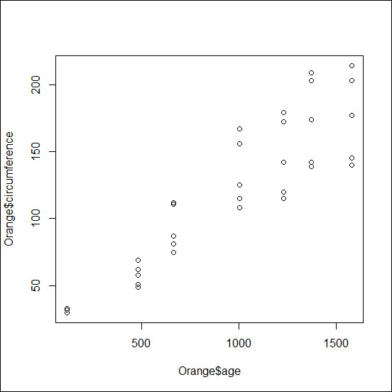
If you want to investigate the relationship between two variables and produce a typical x versus y plot, you can do that with the plot() function. As an example, we can use the dataset Orange and produce a plot of the age versus circumference values for the orange trees:

> plot(Orange$age,Orange$circumference)

Other basic plots available are, for instance, histograms, with the function histogram(), the bar plot, with the function barplot(), and pie charts, with the function piegraph().

The previous code will lead to the output as shown in the following image. Within the plot() function, you can specify other optional arguments in order to modify the basic plot and change its look and/or add information to the figure. The following is a list of the main functions:

On top of the main plot, which is defined by a high-level function (plot() in this case), you may add additional components using low-level functions, such as points for points or lines for lines. The following screenshot shows a simple x-y plot with the dataset Orange:

The following is an example of how to specify these options in plot:.

plot(Orange$age,Orange$circumference, 
    main="Plot of Orange dataset",
    xlab="Age",
    ylab="Circumference",
    type="p",
    pch=2,
    col="red")
lines(loess.smooth(Orange$age,Orange$circumference), 
      col="blue",
      lwd=2)

The output of this plot is reported in the following screenshot:

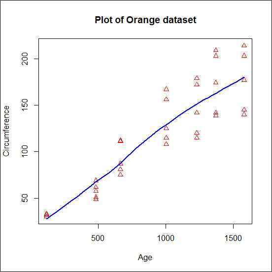
In the previous example, we used the plot() function to generate the first plot containing the individual observation, and then we used the lines() function to add a line representing the tendency of the data. The function loess.smooth() computes the point of a smooth curve, a curve describing the tendency of the data, and these points are then passed to the function lines that draws them in the plot. You can have an idea of the output produced by the loess.smooth() function by running the following code:

> loess.smooth(Orange$age,Orange$circumference)