

In the previous recipe, we familiarized ourselves with heat map functions in R using built-in data. Now, we will learn how to use external data to create our heat maps.
In real life, we often have no control over the format of the data files that we download, or the data that is the output of a particular program. Because we can not always rely on luck that the data comes in the right format, we will learn in this recipe how to read in data from different file formats and get it into shape.
The following image shows a heat map that we are going to create from the gene_expression.txt data set in this recipe:

Download the script 5644OS_02_01.r and the data sets gene_expression.txt, runners.csv, and apple_stocks.xlsx from your account at http://www.packtpub.com and save them to your hard drive.
I recommend that you download and save the script and data files to the same folder on your hard drive. If you execute the script from a different location to the location of the data files, you have to change the current R working directory accordingly.
Tip
You can change the current working directory of your R session by using the setwd() function. If you saved the data files for this recipe under /home/user/Downloads, for example, you would type setwd("/home/user/Downloads") into the R command-line. Alternatively, you can uncomment the fourth line of the script and provide the location of the data file directory to the setwd() function in a similar way.
For more information on how to view the current working directory of your current R session and an explanation on how to run scripts in R, please read the Getting ready section of the Creating your first heat map in R recipe.
After you have executed the following code from the 5644OS_02_01.r script, take a look at the PDF file readingData.pdf, which was created in the same location where you executed the script:
# if you are running the script from a different location
# than the location of the data sets, uncomment the
# next line and point setwd() to the data set location
# setwd("/home/username/Datasets")

### loading packages
if (!require("gplots")) {
install.packages("gplots", dependencies = TRUE)
library(gplots)
}
if (!require("lattice")) {
install.packages("lattice", dependencies = TRUE)
library(lattice)
}
if (!require("xlsx")) {
install.packages("xlsx", dependencies = TRUE)
library(xlsx)
}

pdf("readingData.pdf")

### loading data and drawing heat maps

# 1) gene_expression.txt
gene_data <- read.table("gene_expression.txt",
  comment.char = "/",
  blank.lines.skip = TRUE,
  header = TRUE,
  sep = "\t",
  nrows = 20)
gene_data <- data.matrix(gene_data)
gene_ratio <- outer(gene_data[,"Treatment"],
  gene_data[,"Control"],
  FUN = "/")
heatmap.2(gene_ratio,
  xlab = "Control",
  ylab = "Treatment",
  trace = "none",
  main = "gene_expression.txt")

# 2) runners.csv
runner_data <- read.csv("runners.csv")
rownames(runner_data) <- runner_data[,1]
runner_data <- data.matrix(runner_data[,2:ncol(runner_data)])
colnames(runner_data) <- c(2003:2012)
runner_data[runner_data == 0.00] <- NA
heatmap.2(runner_data,
  dendrogram = "none",
  Colv = NA,
  Rowv = NA,
  trace = "none",
  na.color = "gray",
  main = "runners.csv",
  margin = c(8,10))

# 3) apple_stocks.xlsx
stocks_table <- read.xlsx("apple_stocks.xlsx",
  sheetIndex = 1,
  rowIndex = c(1:28),
  colIndex = c(1:5,7))
row_names <- (stocks_table[,1])
stocks_matrix <- data.matrix(
  stocks_table[2:ncol(stocks_table)])
rownames(stocks_matrix) <- as.character(row_names)
stocks_data = t(stocks_matrix)
print(levelplot(stocks_data,
  col.regions = heat.colors,
  margin = c(10,10),
  scales = list(x = list(rot = 90)),
  main = "apple_stocks.xlsx",
  ylab = NULL,
  xlab = NULL))

dev.off()Generally, R is able to read data from any file that contains data in a proper text format. First, we will see how to use the universal read.table() function to read data from a .txt file. Next, the recipe shows us how to read data from a Comma Separated Values (CSV) file using the read.csv() function. And finally, we take a look at the xlsx() function from the xlsx package, in order to process Microsoft Excel spreadsheet files.
Inspecting gene_expression.txt: The first file that reads into R,
gene_expression.txt, contains exemplary gene expression data obtained from two different conditions: control and treatment. The individual values in this data file resemble fold-differences of gene expression relative to a housekeeping gene that was used as a reference to normalize the data.The data was saved as a
.txtfile and consists of 105 lines. The first two lines from the top are comments about the data and begin with a slash (/) as the first character. Followed by two blank lines, a header labels the two data columns of the expression data under the two conditions.Notice that the data columns are separated by tab spaces as shown in the following screenshot of the
gene_expression.txtdata set:
Reading data from gene_expression.txt: Let's take a look at the arguments we need to provide in the
read.table()function in order to read this data file as a data table into R:gene_data <- read.table("gene_expression.txt", comment.char = "/", blank.lines.skip = TRUE, header = TRUE, sep = "\t", nrows = 20)When we use the
read.table()function, R ignores every line in the data file that starts with a hash mark (#), which is the default comment character. However, the first character of the comment lines in our data file is a forward slash (/). Therefore, we have to pass it to the function as an additional argument for thecomment.charparameter so R can interpret the first two lines ingene_expression.txtas comments and skip them. The second argument,blank.lines.skip = TRUE, ensures that R also skips the two blank lines after the comment section.Tip
Alternatively, we could also use the argument
skip = 4to force R to ignore the first four lines in this text file.From here on, R will read every line that follows and will interpret it as data—skipping the comment and blank lines at the beginning.
There are two data columns in this text file, which are labeled as
ControlandTreatment. By setting the header parameter toTRUE, R will store these labels as a header for our data table. The header is followed by 100 rows of tab-delimited data (Gene1toGene100). We need to use the argumentsep = "/t"to set the field separator character to a tab space, since the default data field separator is the white space,sep = "".The data file is quite large with its 100 entries, and for this example, we just use the first 20 genes to create our heat map. We can tell R to stop reading data after the 20th entry by providing the argument
nrows = 20in the function call.Converting the data table into a numerical matrix: As we remember from the Creating your first heat map in R recipe, we need to convert our data into a numeric matrix format before we can use it to create a heat map. Instead of using the relative expression measures deployed in the data file, we are interested in showing the fold-changes of the gene expression levels. To calculate those fold-changes of the
Treatmentcolumn in relation to theControlcolumn, we are using theouter()function. This function allows us to create a 20 x 20 matrix by dividing each gene from theTreatmentcolumn (third column in the data file) by each gene from theControlcolumn (second column in the data file):gene_data <- data.matrix(gene_data) gene_ratio <- outer(gene_data[,"Treatment"], gene_data[,"Control"], FUN = "/")
Reading data from runners.csv: The
runners.csvfile contains the fastest personal times of seven popular 100 meters sprinters for the years between 2003 and 2012.If we want to read a data file with comma-separated values, it is most convenient to use the
read.csv()function:runner_data <- read.csv("runners.csv")Dealing with missing values in runners.csv: The default constant for missing values in R is
NA, which stands forNot Available. Therefore, if we read data from a file that contains empty fields, missing values will be replaced byNAwhen R creates the data table.When we read in
runner_data.csv, we see that our data table contains many0.00values, which means that no time was recorded for the runner in those years. However, it would make more sense to have those values denoted as missing data (NA) in our heat map.So, if we want R to interpret values other than
NAor empty fields as missing values, we do this by providing an argument for thena.stringsparameter in ourread.table()orread.csv()function:runner_data <- read.csv("runners.csv", na.strings = 0.00)Note
We can convert also particular data in the table to missing values after we read it from a file. In our case, we could use the following command to convert all
0.00data points to missing values:runner_data[runner_data == 0.00] <- NABy default, cells with
NAvalues will be left blank and appear as white cells in our heat map. This can be very misleading, since the color palette that we are using converges into a very bright yellow. It would be very hard to distinguish those empty cells from values that are seeded very high in our color key.To avoid this confusion, we can simply assign a different color to those cells that contain missing values. Here, we are coloring them in gray:
heatmap.2(runner_data, dendrogram = "none", Colv = NA, Rowv = NA, trace = "none", na.color = "gray", main = "runners.csv", margin = c(8,10))Reading Apple's stock data from an Excel spreadsheet file: Now, let us take a look at Apple's daily stock market data from 1984 to 2013.
The following screenshot shows the
apple_stock.xlsxdata set opened in Microsoft Excel 2011:
R has no in-built function to read data from this proprietary format. But, we are lucky that someone developed the
xlsxpackage especially for this case that is freely available on CRAN. Therefore, we can use theread.xlsx()function to conveniently get this data fromapple_stock.xlsxinto R.stocks_table <- read.xlsx("apple_stocks.xlsx", sheetIndex = 1, rowIndex = c(1:28), colIndex = c(1:5,7))With
sheetIndex, we have selected which sheet we want to read from the Excel spreadsheet file—apple_stock.xlsxonly has data onsheet 1. The spreadsheet consists of 7168 rows of data, but we are interested only in the recent data stock data of 2013. So, to only read in those first 28 lines, we included therowIndex = c(1:28)argument in theread.xlsx()function call above. Furthermore, we are not interested in theVolumecolumn (column 6), so let's skip it via the argumentcolIndex = c(1:5,7).Note
You can also use the
read.xlsx()function to read data from the old Excel spreadsheet format.xls.In most cases, we will use the
read.table()function to read our data into R. The following table summarizes the most important options: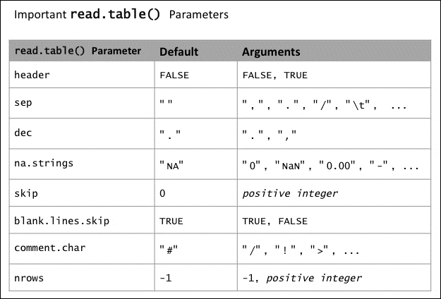
It might happen that we obtain our data in the so-called long format, which contains multiple rows for each individual category, individual or item.
To give you a better understanding, an excerpt from the runners.csv data set in long format is shown as follows:
  Year       Runner  Time
1 2007   Usain_Bolt 10.03
2 2008   Usain_Bolt  9.72
3 2009   Usain_Bolt  9.58
4 2010   Usain_Bolt  9.82
5 2011   Usain_Bolt  9.76
6 2012   Usain_Bolt  9.63
7 2004 Asafa_Powell 10.02
8 2005 Asafa_Powell  9.87
...
Do you see the problem here? The Runner column in the middle of the data table consists of character strings, which are incompatible with the numeric matrix format that is required by our heat map functions.
Fortunately, it is quite easy to convert data from long to wide format—we can simply use the cross tabulation function xtabs():
runners_wide <- xtabs(formula = Time ~ Runner + Year, data =
runners_long))

              Year
Runner          2004  2005  2007  2008  2009  2010  2011  2012
  Asafa_Powell 10.02  9.87  0.00  0.00  0.00  0.00  0.00  0.00
  Usain_Bolt    0.00  0.00 10.03  9.72  9.58  9.82  9.76  9.63
Tip
If you just want to transpose your data, that is, switch columns and rows, you can use the t() function:
transposed_data <- t(my_data)
Several countries use a decimal comma instead of a decimal point. Chances are high that you want to analyze a data set that comes from one of those countries. In this case you just have to provide an additional argument for the dec parameter:
my_data <- read.table("data.txt", dec=",")