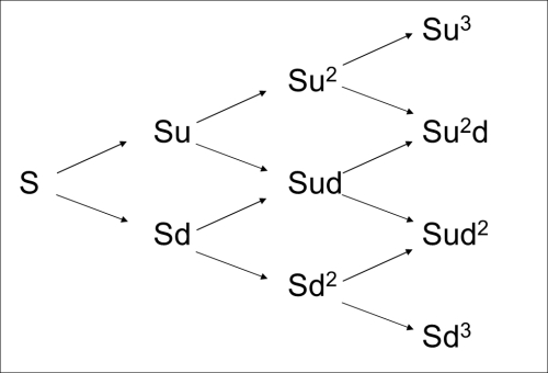
The Cox-Ross-Rubinstein (CRR) model (Cox, Ross and Rubinstein, 1979) assumes that the price of the underlying asset follows a discrete binomial process. The price might go up or down in each period and hence changes according to a binomial tree illustrated in the following plot, where u and d are fixed multipliers measuring the price changes when it goes up and down. The important feature of the CRR model is that u=1/d and the tree is recombining; that is, the price after two periods will be the same if it first goes up and then goes down or vice versa, as shown in the following figure:

To build a binomial tree, first we have to decide how many steps we are modeling (n); that is, how many steps the time to maturity of the option will be divided into. Alternatively, we can determine the length of one time step t, (measured in years) on the tree:

If we know the volatility (σ) of the underlying, the parameters u and d are determined according to the following formulas...