
The notebook is the flagship feature of IPython. This web-based interactive environment combines code, rich text, images, videos, animations, mathematics, and plots into a single document. This modern tool is an ideal gateway to high-performance numerical computing and data science in Python. This entire book has been written in the notebook, and the code of every recipe is available as a notebook on the book's GitHub repository at https://github.com/ipython-books/cookbook-code.
In this recipe, we give an introduction to IPython and its notebook. In Getting ready, we also give general instructions on installing IPython and the Python scientific stack.
You will need Python, IPython, NumPy, pandas, and matplotlib in this chapter. Together with SciPy and SymPy, these libraries form the core of the Python scientific stack (www.scipy.org/about.html).
Note
You will find full detailed installation instructions on the book's GitHub repository at https://github.com/ipython-books/cookbook-code.
We only give a summary of these instructions here; please refer to the link above for more up-to-date details.
If you're just getting started with scientific computing in Python, the simplest option is to install an all-in-one Python distribution. The most common distributions are:
Anaconda (free or commercial license) available at http://store.continuum.io/cshop/anaconda/
Canopy (free or commercial license) available at www.enthought.com/products/canopy/
Python(x,y), a free distribution only for Windows, available at https://code.google.com/p/pythonxy/
We highly recommend Anaconda. These distributions contain everything you need to get started. You can also install additional packages as needed. You will find all the installation instructions in the links mentioned previously.
Note
Throughout the book, we assume that you have installed Anaconda. We may not be able to offer support to readers who use another distribution.
Alternatively, if you feel brave, you can install Python, IPython, NumPy, pandas, and matplotlib manually. You will find all the instructions on the following websites:
Python is the programming language underlying the ecosystem. The instructions are available at www.python.org/.
IPython provides tools for interactive computing in Python. The instructions for installation are available at http://ipython.org/install.html.
NumPy/SciPy are used for numerical computing in Python. The instructions for installation are available at www.scipy.org/install.html.
pandas provides data structures and tools for data analysis in Python. The instructions for installation are available at http://pandas.pydata.org/getpandas.html.
matplotlib helps in creating scientific figures in Python. The instructions for installation are available at http://matplotlib.org/index.html.
Note
Python 2 or Python 3?
Though Python 3 is the latest version at this date, many people are still using Python 2. Python 3 has brought backward-incompatible changes that have slowed down its adoption. If you are just getting started with Python for scientific computing, you might as well choose Python 3. In this book, all the code has been written for Python 3, but it also works with Python 2. We will give more details about this question in Chapter 2, Best Practices in Interactive Computing.
Once you have installed either an all-in-one Python distribution (again, we highly recommend Anaconda), or Python and the required packages, you can get started! In this book, the IPython notebook is used in almost all recipes. This tool gives you access to Python from your web browser. We covered the essentials of the notebook in the Learning IPython for Interactive Computing and Data Visualization book. You can also find more information on IPython's website (http://ipython.org/ipython-doc/stable/notebook/index.html).
To run the IPython notebook server, type ipython notebook in a terminal (also called the command prompt). Your default web browser should open automatically and load the 127.0.0.1:8888 address. Then, you can create a new notebook in the dashboard or open an existing notebook. By default, the notebook server opens in the current directory (the directory you launched the command from). It lists all the notebooks present in this directory (files with the .ipynb extension).
We assume that a Python distribution is installed with IPython and that we are now in an IPython notebook. We type the following command in a cell, and press Shift + Enter to evaluate it:
In [1]: print("Hello world!")
Hello world!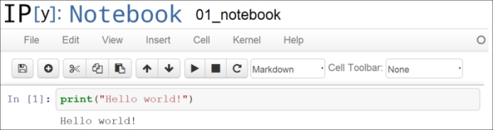
Screenshot of the IPython notebook
A notebook contains a linear succession of cells and output areas. A cell contains Python code, in one or multiple lines. The output of the code is shown in the corresponding output area.
Now, we do a simple arithmetic operation:
In [2]: 2+2
Out[2]: 4
The result of the operation is shown in the output area. Let's be more precise. The output area not only displays the text that is printed by any command in the cell, but it also displays a text representation of the last returned object. Here, the last returned object is the result of
2+2, that is,4.In the next cell, we can recover the value of the last returned object with the
_(underscore) special variable. In practice, it might be more convenient to assign objects to named variables such as inmyresult = 2+2.In [3]: _ * 3 Out[3]: 12
IPython not only accepts Python code, but also shell commands. These commands are defined by the operating system (mainly Windows, Linux, and Mac OS X). We first type
!in a cell before typing the shell command. Here, assuming a Linux or Mac OS X system, we get the list of all the notebooks in the current directory:In [4]: !ls *.ipynb notebook1.ipynb ...
On Windows, you should replace
lswithdir.IPython comes with a library of magic commands. These commands are convenient shortcuts to common actions. They all start with
%(the percent character). We can get the list of all magic commands with%lsmagic:In [5]: %lsmagic Out[5]: Available line magics: %alias %alias_magic %autocall %automagic %autosave %bookmark %cd %clear %cls %colors %config %connect_info %copy %ddir %debug %dhist %dirs %doctest_mode %echo %ed %edit %env %gui %hist %history %install_default_config %install_ext %install_profiles %killbgscripts %ldir %less %load %load_ext %loadpy %logoff %logon %logstart %logstate %logstop %ls %lsmagic %macro %magic %matplotlib %mkdir %more %notebook %page %pastebin %pdb %pdef %pdoc %pfile %pinfo %pinfo2 %popd %pprint %precision %profile %prun %psearch %psource %pushd %pwd %pycat %pylab %qtconsole %quickref %recall %rehashx %reload_ext %ren %rep %rerun %reset %reset_selective %rmdir %run %save %sc %store %sx %system %tb %time %timeit %unalias %unload_ext %who %who_ls %whos %xdel %xmode Available cell magics: %%! %%HTML %%SVG %%bash %%capture %%cmd %%debug %%file %%html %%javascript %%latex %%perl %%powershell %%prun %%pypy %%python %%python3 %%ruby %%script %%sh %%svg %%sx %%system %%time %%timeit %%writefile
Cell magics have a
%%prefix; they concern entire code cells.For example, the
%%writefilecell magic lets us create a text file easily. This magic command accepts a filename as an argument. All the remaining lines in the cell are directly written to this text file. Here, we create a filetest.txtand writeHello world!in it:In [6]: %%writefile test.txt Hello world! Writing test.txt In [7]: # Let's check what this file contains. with open('test.txt', 'r') as f: print(f.read()) Hello world!As we can see in the output of
%lsmagic, there are many magic commands in IPython. We can find more information about any command by adding?after it. For example, to get some help about the%runmagic command, we type%run?as shown here:In [9]: %run? Type: Magic function Namespace: IPython internal ... Docstring: Run the named file inside IPython as a program. [full documentation of the magic command...]
We covered the basics of IPython and the notebook. Let's now turn to the rich display and interactive features of the notebook. Until now, we have only created code cells (containing code). IPython supports other types of cells. In the notebook toolbar, there is a drop-down menu to select the cell's type. The most common cell type after the code cell is the Markdown cell.
Markdown cells contain rich text formatted with Markdown, a popular plain text-formatting syntax. This format supports normal text, headers, bold, italics, hypertext links, images, mathematical equations in LaTeX (a typesetting system adapted to mathematics), code, HTML elements, and other features, as shown here:
### New paragraph This is *rich* **text** with [links](http://ipython.org), equations: $$\hat{f}(\xi) = \int_{-\infty}^{+\infty} f(x)\, \mathrm{e}^{-i \xi x}$$ code with syntax highlighting: ```python print("Hello world!") ``` and images: Running a Markdown cell (by pressing Shift + Enter, for example) displays the output, as shown in the following screenshot:

Rich text formatting with Markdown in the IPython notebook
Note
LaTeX equations are rendered with the
MathJaxlibrary. We can enter inline equations with$...$and displayed equations with$$...$$. We can also use environments such asequation,eqnarray, oralign. These features are very useful to scientific users.By combining code cells and Markdown cells, we can create a standalone interactive document that combines computations (code), text, and graphics.
IPython also comes with a sophisticated display system that lets us insert rich web elements in the notebook. Here, we show how to add HTML, SVG (Scalable Vector Graphics), and even YouTube videos in a notebook.
First, we need to import some classes:
In [11]: from IPython.display import HTML, SVG, YouTubeVideo
We create an HTML table dynamically with Python, and we display it in the notebook:
In [12]: HTML('''
         <table style="border: 2px solid black;">
         ''' +
         ''.join(['<tr>' +
                  ''.join(['<td>{row},{col}</td>'.format(
                                 row=row, col=col
                                 ) for col in range(5)]) +
                  '</tr>' for row in range(5)]) +
         '''
         </table>
         ''')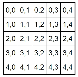
An HTML table in the notebook
Similarly, we can create SVG graphics dynamically:
In [13]: SVG('''<svg width="600" height="80">''' +
         ''.join(['''<circle cx="{x}" cy="{y}" r="{r}"
                             fill="red"
                             stroke-width="2"
                             stroke="black">
                     </circle>'''.format(x=(30+3*i)*(10-i),
                                         y=30,
                                         r=3.*float(i)
                                         ) for i in range(10)]) +
         '''</svg>''')
SVG in the notebook
Finally, we display a YouTube video by giving its identifier to
YoutubeVideo:In [14]: YouTubeVideo('j9YpkSX7NNM')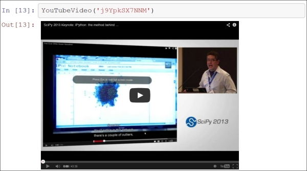
YouTube in the notebook
Now, we illustrate the latest interactive features in IPython 2.0+, namely JavaScript widgets. Here, we create a drop-down menu to select videos:
In [15]: from collections import OrderedDict
         from IPython.display import (display,
                                      clear_output,
                                      YouTubeVideo)
         from IPython.html.widgets import DropdownWidget
In [16]: # We create a DropdownWidget, with a dictionary
         # containing the keys (video name) and the values
         # (Youtube identifier) of every menu item.
         dw = DropdownWidget(values=OrderedDict([
                           ('SciPy 2012', 'iwVvqwLDsJo'),
                           ('PyCon 2012', '2G5YTlheCbw'),
                           ('SciPy 2013', 'j9YpkSX7NNM')]
                                                )
                             )

         # We create a callback function that displays the
         # requested Youtube video.
         def on_value_change(name, val):
             clear_output()
             display(YouTubeVideo(val))

         # Every time the user selects an item, the
         # function `on_value_change` is called, and the
         # `val` argument contains the value of the selected
         # item.
         dw.on_trait_change(on_value_change, 'value')

         # We choose a default value.
         dw.value = dw.values['SciPy 2013']

         # Finally, we display the widget.
         display(dw)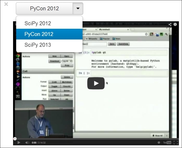
An interactive widget in the notebook
The interactive features of IPython 2.0 bring a whole new dimension to the notebook, and we can expect many developments in the future.
Notebooks are saved as structured text files (JSON format), which makes them easily shareable. Here are the contents of a simple notebook:
{
 "metadata": {
  "name": ""
 },
 "nbformat": 3,
 "nbformat_minor": 0,
 "worksheets": [
  {
   "cells": [
    {
     "cell_type": "code",
     "collapsed": false,
     "input": [
      "print(\"Hello World!\")"
     ],
     "language": "python",
     "metadata": {},
     "outputs": [
      {
       "output_type": "stream",
       "stream": "stdout",
       "text": [
        "Hello World!\n"
       ]
      }
     ],
     "prompt_number": 1
    }
   ],
   "metadata": {}
  }
 ]
}
IPython comes with a special tool, nbconvert, which converts notebooks to other formats such as HTML and PDF (http://ipython.org/ipython-doc/stable/notebook/index.html).
Another online tool, nbviewer, allows us to render a publicly available notebook directly in the browser and is available at http://nbviewer.ipython.org.
We will cover many of these possibilities in the subsequent chapters, notably in Chapter 3, Mastering the Notebook.
Here are a few references about the notebook:
Official page of the notebook available at http://ipython.org/notebook
Documentation of the notebook available at http://ipython.org/ipython-doc/dev/notebook/index.html
Official notebook examples present at https://github.com/ipython/ipython/tree/master/examples/Notebook
User-curated gallery of interesting notebooks available at https://github.com/ipython/ipython/wiki/A-gallery-of-interesting-IPython-Notebooks
Official tutorial on the interactive widgets present at http://nbviewer.ipython.org/github/ipython/ipython/tree/master/examples/Interactive%20Widgets/