
It is a well-known and commonly accepted stylized fact in empirical finance that the volatility of financial time series varies over time. However, the non-observable nature of volatility makes the measurement and forecasting a challenging exercise. Usually, varying volatility models are motivated by three empirical observations:
Volatility clustering: This refers to the empirical observation that calm periods are usually followed by calm periods while turbulent periods by turbulent periods in the financial markets.
Non-normality of asset returns: Empirical analysis has shown that asset returns tend to have fat tails relative to the normal distribution.
Leverage effect: This leads to an observation that volatility tends to react differently to positive or negative price movements; a drop in prices increases the volatility to a larger extent than an increase of similar size.
In the following code, we demonstrate these stylized facts based on S&P asset prices. Data is downloaded from yahoofinance, by using the already known method:
getSymbols("SNP", from="2004-01-01", to=Sys.Date())
chartSeries(Cl(SNP))
Our purpose of interest is the daily return series, so we calculate log returns from the closing prices. Although it is a straightforward calculation, the Quantmod package offers an even simpler way:
ret <- dailyReturn(Cl(SNP), type='log')
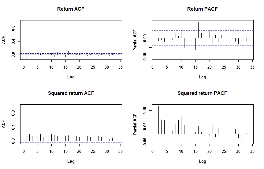
Volatility analysis departs from eyeballing the autocorrelation and partial autocorrelation functions. We expect the log returns to be serially uncorrelated, but the squared or absolute log returns to show significant autocorrelations. This means that Log returns are not correlated, but not independent.
Notice the par(mfrow=c(2,2)) function in the following code; by this, we overwrite the default plotting parameters of R to organize the four diagrams of interest in a convenient table format:
par(mfrow=c(2,2))
acf(ret, main="Return ACF");
pacf(ret, main="Return PACF");
acf(ret^2, main="Squared return ACF");
pacf(ret^2, main="Squared return PACF")
par(mfrow=c(1,1))
The screenshot for preceding command is as follows:
Next, we look at the histogram and/or the empirical distribution of daily log returns of S&P and compare it with the normal distribution of the same mean and standard deviation. For the latter, we use the function density(ret), which computes the nonparametric empirical distribution function. We use the function curve()with an additional parameter add=TRUE to plot a second line to an already existing diagram:
m=mean(ret);s=sd(ret);
par(mfrow=c(1,2))
hist(ret, nclass=40, freq=FALSE, main='Return histogram');curve(dnorm(x, mean=m,sd=s), from = -0.3, to = 0.2, add=TRUE, col="red")
plot(density(ret), main='Return empirical distribution');curve(dnorm(x, mean=m,sd=s), from = -0.3, to = 0.2, add=TRUE, col="red")
par(mfrow=c(1,1))
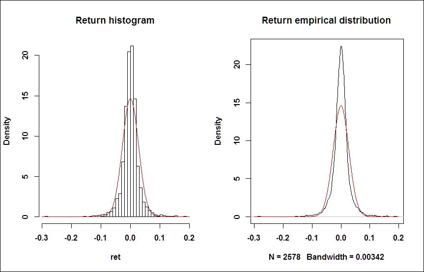
The excess kurtosis and fat tails are obvious, but we can confirm numerically (using the moments package) that the kurtosis of the empirical distribution of our sample exceeds that of a normal distribution (which is equal to 3). Unlike some other software packages, R reports the nominal value of kurtosis, and not excess kurtosis which is as follows:
> kurtosis(ret)
daily.returns
     12.64959
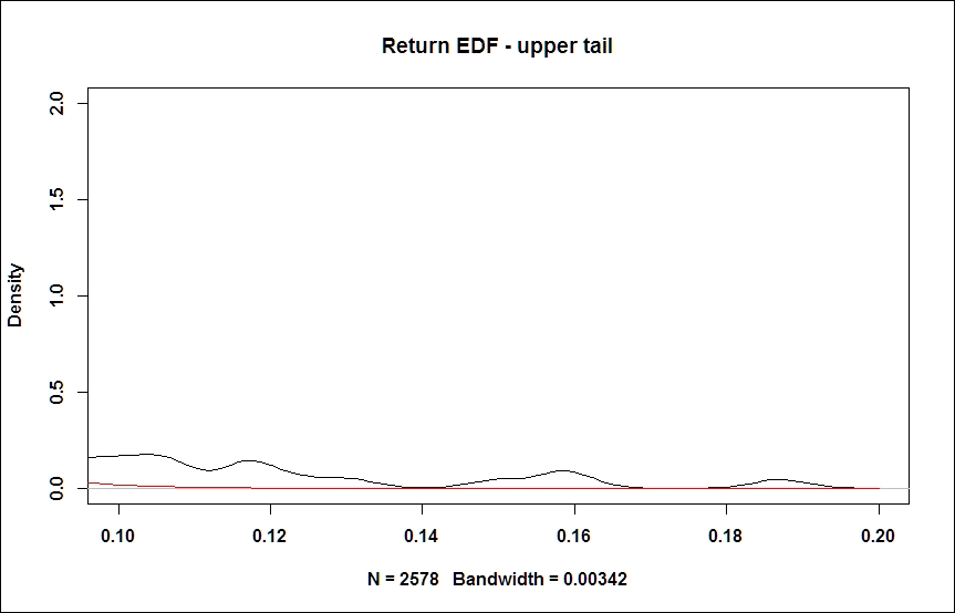
It might be also useful to zoom in to the upper or the lower tail of the diagram. This is achieved by simply rescaling our diagrams:
# tail zoom
plot(density(ret), main='Return EDF - upper tail', xlim = c(0.1, 0.2), ylim=c(0,2));
curve(dnorm(x, mean=m,sd=s), from = -0.3, to = 0.2, add=TRUE, col="red")
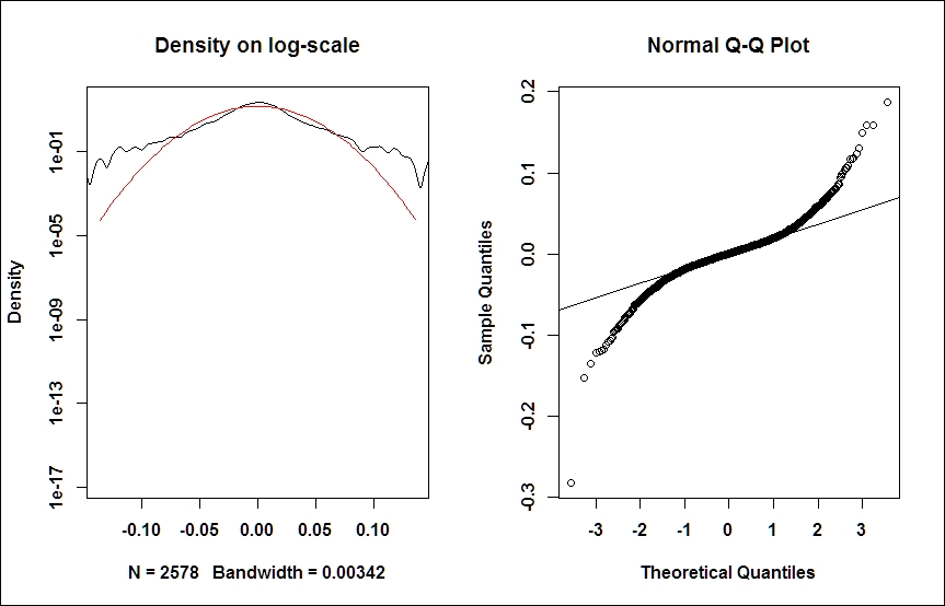
Another useful visualization exercise is to look at the Density on log-scale (see the following figure, left), or a QQ-plot (right), which are common tools to comparing densities. QQ-plot depicts the empirical quantiles against that of a theoretical (normal) distribution. In case our sample is taken from a normal distribution, this should form a straight line. Deviations from this straight line may indicate the presence of fat tails:
# density plots on log-scale
plot(density(ret), xlim=c(-5*s,5*s),log='y', main='Density on log-scale')
curve(dnorm(x, mean=m,sd=s), from=-5*s, to=5*s, log="y", add=TRUE, col="red")

# QQ-plot
qqnorm(ret);qqline(ret);
The screenshot for preceding command is as follows:
Now, we can turn our attention to modeling volatility.
Broadly speaking, there are two types of modeling techniques in the financial econometrics literature to capture the varying nature of volatility: the GARCH-family approach (Engle, 1982 and Bollerslev, 1986) and the stochastic volatility (SV) models. As for the distinction between them, the main difference between the GARCH-type modeling and (genuine) SV-type modeling techniques is that in the former, the conditional variance given in the past observations is available, while in SV-models, volatility is not measurable with respect to the available information set; therefore, it is hidden by nature, and must be filtered out from the measurement equation (see, for example, Andersen – Benzoni (2011)). In other words, GARCH-type models involve the estimation of volatility based on past observations, while in SV-models, the volatility has its own stochastic process, which is hidden, and return realizations should be used as a measurement equation to make inferences regarding the underlying volatility process.
In this chapter, we introduce the basic modeling techniques for the GARCH approach for two reasons; first of all, it is much more proliferated in applied works. Secondly, because of its diverse methodological background, SV models are not yet supported by R packages natively, and a significant amount of custom development is required for an empirical implementation.
There are several packages available in R for GARCH modeling. The most prominent ones are rugarch, rmgarch (for multivariate models), and fGarch; however, the basic tseries package also includes some GARCH functionalities. In this chapter, we will demonstrate the modeling facilities of the rugarch package. Our notations in this chapter follow the respective ones of the rugarch package's output and documentation.
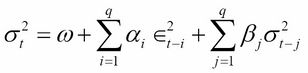
A GARCH (p,q) process may be written as follows:

Here,  is usually the disturbance term of a conditional mean equation (in practice, usually an ARMA process) and
  . That is, the conditional volatility process is determined linearly by its own lagged values
  and the lagged squared observations (the values of ). In empirical studies, GARCH (1,1) usually provides an appropriate fit to the data. It may be useful to think about the simple GARCH (1,1) specification as a model in which the conditional variance is specified as a weighted average of the long-run variance
  , the last predicted variance
  , and the new information
  (see Andersen et al. (2009)). It is easy to see how the GARCH (1,1) model captures autoregression in volatility (volatility clustering) and leptokurtic asset return distributions, but as its main drawback, it is symmetric, and cannot capture asymmetries in distributions and leverage effects.
The emergence of volatility clustering in a GARCH-model is highly intuitive; a large positive (negative) shock in  increases (decreases) the value of , which in turn increases (decreases) the value of
  , resulting in a larger (smaller) value for
  . The shock is persistent; this is volatility clustering. Leptokurtic nature requires some derivation; see for example Tsay (2010).
Our empirical example will be the analysis of the return series calculated from the daily closing prices of Apple Inc. based on the period from Jan 01, 2006 to March 31, 2014. As a useful exercise, before starting this analysis, we recommend that you repeat the exploratory data analysis in this chapter to identify stylized facts on Apple data.
Obviously, our first step is to install a package, if not installed yet:
install.packages('rugarch');library('rugarch')
To get the data, as usual, we use the quantmod package and the getSymbols() function, and calculate return series based on the closing prices.
#Load Apple data and calculate log-returns
getSymbols("AAPL", from="2006-01-01", to="2014-03-31")
ret.aapl <- dailyReturn(Cl(AAPL), type='log')
chartSeries(ret.aapl)
The programming logic of rugarch can be thought of as follows: irrespective of whatever your aim is (fitting, filtering, forecasting, and simulating), first, you have to specify a model as a system object (variable), which in turn will be inserted into the respective function. Models can be specified by calling ugarchspec(). The following code specifies a simple GARCH (1,1) model, (sGARCH), with only a constant  in the mean equation:
garch11.spec = ugarchspec(variance.model = list(model="sGARCH", garchOrder=c(1,1)), mean.model = list(armaOrder=c(0,0)))
An obvious way to proceed is to fit this model to our data, that is, to estimate the unknown parameters by maximum likelihood, based on our time series of daily returns:
aapl.garch11.fit = ugarchfit(spec=garch11.spec, data=ret.aapl)
The function provides, among a number of other outputs, the parameter estimations  :
:
> coef(aapl.garch11.fit)
          mu        omega       alpha1        beta1
1.923328e-03 1.027753e-05 8.191681e-02 8.987108e-01
Estimates and various diagnostic tests can be obtained by the show() method of the generated object (that is, by just typing the name of the variable). A bunch of other statistics, parameter estimates, standard error, and covariance matrix estimates can be reached by typing the appropriate command. For the full list, consult the ugarchfit object class; the most important ones are shown in the following code:
coef(msft.garch11.fit)          #estimated coefficients
vcov(msft.garch11.fit)          #covariance matrix of param estimates
infocriteria(msft.garch11.fit)  #common information criteria list
newsimpact(msft.garch11.fit)    #calculate news impact curve
signbias(msft.garch11.fit)      #Engle - Ng sign bias test
fitted(msft.garch11.fit)        #obtain the fitted data series
residuals(msft.garch11.fit)     #obtain the residuals
uncvariance(msft.garch11.fit)   #unconditional (long-run) variance
uncmean(msft.garch11.fit)       #unconditional (long-run) mean
Standard GARCH models are able to capture fat tails and volatility clustering, but to explain asymmetries caused by the leverage effect, we need more advanced models. To approach the asymmetry problem visually, we will now describe the concept of news impact curves.
News impact curves, introduced by Pagan and Schwert (1990) and Engle and Ng (1991), are useful tools to visualize the magnitude of volatility changes in response to shocks. The name comes from the usual interpretation of shocks as news influencing the market movements. They plot the change in conditional volatility against shocks in different sizes, and can concisely express the asymmetric effects in volatility. In the following code, the first line calculates the news impacts numerically for the previously defined GARCH(1,1) model, and the second line creates the visual plot:
ni.garch11 <- newsimpact(aapl.garch11.fit)
plot(ni.garch11$zx, ni.garch11$zy, type="l", lwd=2, col="blue", main="GARCH(1,1) - News Impact", ylab=ni.garch11$yexpr, xlab=ni.garch11$xexpr)
The screenshot for the preceding command is as follows:
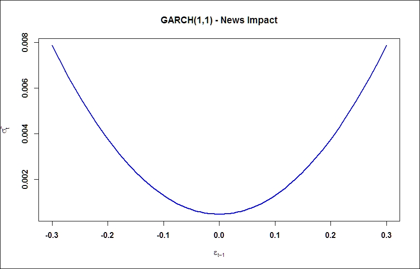
As we expected, no asymmetries are present in response to positive and negative shocks. Now, we turn to models to be able to incorporate asymmetric effects as well.
Exponential GARCH models were introduced by Nelson (1991). This approach directly models the logarithm of the conditional volatility:
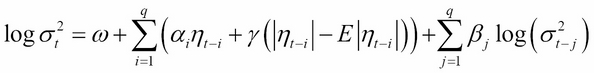
where, E is the expectation operator. This model formulation allows multiplicative dynamics in evolving the volatility process. Asymmetry is captured by the  parameter; a negative value indicates that the process reacts more to negative shocks, as observable in real data sets.
To fit an EGARCH model, the only parameter to be changed in a model specification is to set the EGARCH model type. By running the fitting function, the additional parameter will be estimated (see coef()):
# specify EGARCH(1,1) model with only constant in mean equation
egarch11.spec = ugarchspec(variance.model = list(model="eGARCH", garchOrder=c(1,1)), mean.model = list(armaOrder=c(0,0)))
aapl.egarch11.fit = ugarchfit(spec=egarch11.spec, data=ret.aapl)

> coef(aapl.egarch11.fit)
          mu        omega       alpha1        beta1       gamma1
 0.001446685 -0.291271433 -0.092855672  0.961968640  0.176796061
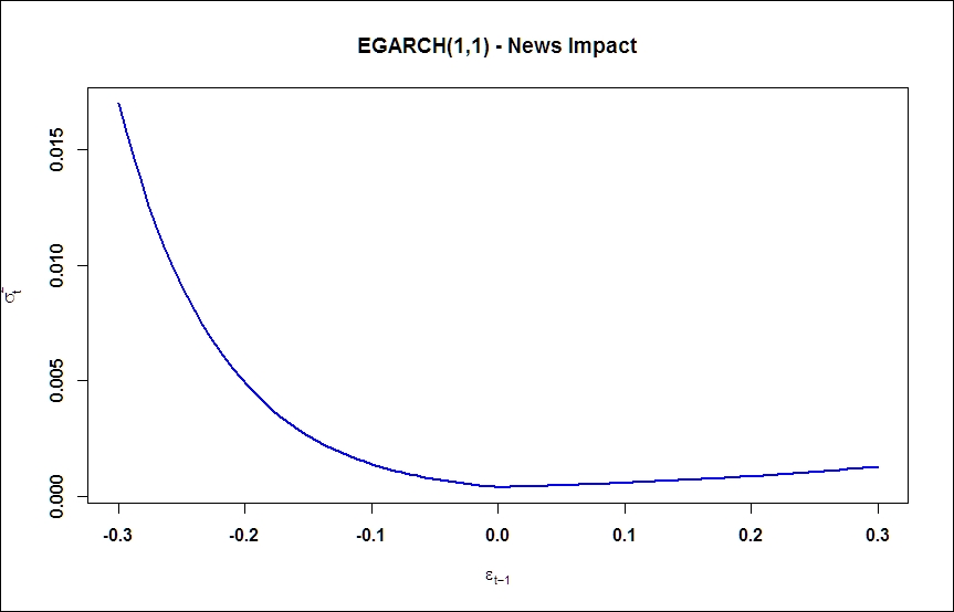
News impact curve reflects the strong asymmetry in response of conditional volatility to shocks and confirms the necessity of asymmetric models:
ni.egarch11 <- newsimpact(aapl.egarch11.fit)
plot(ni.egarch11$zx, ni.egarch11$zy, type="l", lwd=2, col="blue", main="EGARCH(1,1) - News Impact",
ylab=ni.egarch11$yexpr, xlab=ni.egarch11$xexpr)
Another prominent example is the TGARCH model, which is even easier to interpret. The TGARCH specification involves an explicit distinction of model parameters above and below a certain threshold. TGARCH is also a submodel of a more general class, the asymmetric power ARCH class, but we will discuss it separately because of its wide penetration in applied financial econometrics literature.
The TGARCH model may be formulated as follows:
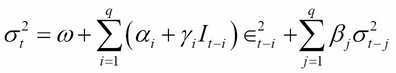
where 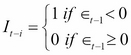
The interpretation is straightforward; the ARCH coefficient depends on the sign of the previous error term; if  is positive, a negative error term will have a higher impact on the conditional volatility, just as we have seen in the leverage effect before.
In the R package, rugarch, the threshold GARCH model is implemented in a framework of an even more general class of GARCH models, called the Family GARCH model Ghalanos (2014).
# specify TGARCH(1,1) model with only constant in mean equation
tgarch11.spec = ugarchspec(variance.model = list(model="fGARCH", submodel="TGARCH", garchOrder=c(1,1)),
          mean.model = list(armaOrder=c(0,0)))
aapl.tgarch11.fit = ugarchfit(spec=tgarch11.spec, data=ret.aapl)

> coef(aapl.egarch11.fit)
          mu        omega       alpha1        beta1       gamma1
 0.001446685 -0.291271433 -0.092855672  0.961968640  0.176796061
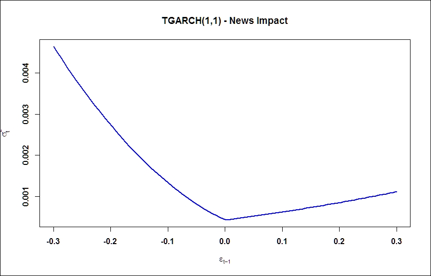
Thanks to the specific functional form, the news impact curve for a Threshold-GARCH is less flexible in representing different responses, there is a kink at the zero point which can be seen when we run the following command:
ni.tgarch11 <- newsimpact(aapl.tgarch11.fit)
plot(ni.tgarch11$zx, ni.tgarch11$zy, type="l", lwd=2, col="blue", main="TGARCH(1,1) - News Impact",
ylab=ni.tgarch11$yexpr, xlab=ni.tgarch11$xexpr)
The Rugarch package allows an easy way to simulate from a specified model. Of course, for simulation purposes, we should also specify the parameters of the model within ugarchspec(); this could be done by the fixed.pars argument. After specifying the model, we can simulate a time series with a given conditional mean and GARCH specification by using simply the ugarchpath() function:
garch11.spec = ugarchspec(variance.model = list(garchOrder=c(1,1)),
  mean.model = list(armaOrder=c(0,0)),
    fixed.pars=list(mu = 0, omega=0.1, alpha1=0.1,
      beta1 = 0.7))
garch11.sim = ugarchpath(garch11.spec, n.sim=1000)
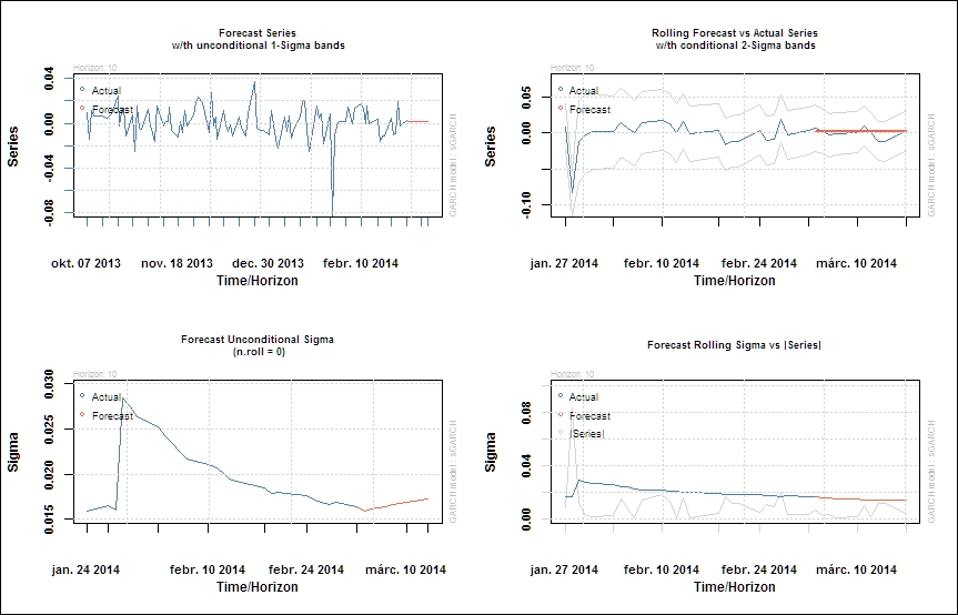
Once we have an estimated model and technically a fitted object, forecasting the conditional volatility based on that is just one step:
aapl.garch11.fit = ugarchfit(spec=garch11.spec, data=ret.aapl, out.sample=20)
aapl.garch11.fcst = ugarchforecast(aapl.garch11.fit, n.ahead=10, n.roll=10)
The plotting method of the forecasted series provides the user with a selection menu; we can plot either the predicted time series or the predicted conditional volatility.
plot(aapl.garch11.fcst, which='all')