The purpose of this example is to check whether everything is working in your installation and give a flavor of what is to come. We concentrate on the Pandas library, which is the main tool used in Python data analysis.

We will use the MovieTweetings 50K movie ratings dataset, which can be downloaded from https://github.com/sidooms/MovieTweetings. The data is from the study MovieTweetings: a Movie Rating Dataset Collected From Twitter - by Dooms, De Pessemier and Martens presented during Workshop on Crowdsourcing and Human Computation for Recommender Systems, CrowdRec at RecSys (2013). The dataset is spread in several text files, but we will only use the following two files:

To see the contents of these files, you can open them with a standard text editor. The data is organized in columns, with one data item per line. The meanings of the columns are described in the README.md file, distributed with the dataset. The data has a peculiar aspect: some of the columns use a double colon (::) character as a separator, while others use a vertical bar (|). This emphasizes a common occurrence with real-world data: we have no control on how the data is collected and formatted. For data stored in text files, such as this one, it is always a good strategy to open the file in a text editor or spreadsheet software to take a look at the data and identify inconsistencies and irregularities.

To read the ratings file, run the following command:

    cols = ['user id', 'item id', 'rating', 'timestamp']
ratings = pd.read_csv('data/ratings.dat', sep='::',
                          index_col=False, names=cols,
                          encoding="UTF-8")

The first line of code creates a Python list with the column names in the dataset. The next command reads the file, using the read_csv() function, which is part of Pandas. This is a generic function to read column-oriented data from text files. The arguments used in the call are as follows:

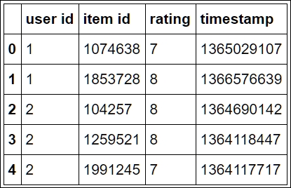
The read_csv() function returns a DataFrame object, which is the Pandas data structure that represents tabular data. We can view the first rows of the data with the following command:

ratings[:5]

This will output a table, as shown in the following image:

To start working with the data, let us find out how many times each rating appears in the table. This can be done with the following commands:

rating_counts = ratings['rating'].value_counts()
rating_counts

The first line of code computes the counts and stores them in the rating_counts variable. To obtain the count, we first use the ratings['rating'] expression to select the rating column from the table ratings. Then, the value_counts() method is called to compute the counts. Notice that we retype the variable name, rating_counts, at the end of the cell. This is a common notebook (and Python) idiom to print the value of a variable in the output area that follows each cell. In a script, it has no effect; we could have printed it with the print command,(print(rating_counts)), as well. The output is displayed in the following image:

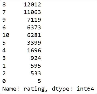
Notice that the output is sorted according to the count values in descending order. The object returned by value_counts is of the Series type, which is the Pandas data structure used to represent one-dimensional, indexed, data. The Series objects are used extensively in Pandas. For example, the columns of a DataFrame object can be thought as Series objects that share a common index.

In our case, it makes more sense to sort the rows according to the ratings. This can be achieved with the following commands:

sorted_counts = rating_counts.sort_index()
sorted_counts

This works by calling the sort_index() method of the Series object, rating_counts. The result is stored in the sorted_counts variable. We can now get a quick visualization of the ratings distribution using the following commands:

sorted_counts.plot(kind='bar', color='SteelBlue')
plt.title('Movie ratings')
plt.xlabel('Rating')
plt.ylabel('Count')

The first line produces the plot by calling the plot() method for the sorted_counts object. We specify the kind='bar' option to produce a bar chart. Notice that we added the color='SteelBlue' option to select the color of the bars in the histogram. SteelBlue is one of the HTML5 color names (for example,  http://matplotlib.org/examples/color/named_colors.html ) available in matplotlib. The next three statements set the title, horizontal axis label, and vertical axis label respectively. This will produce the following plot:

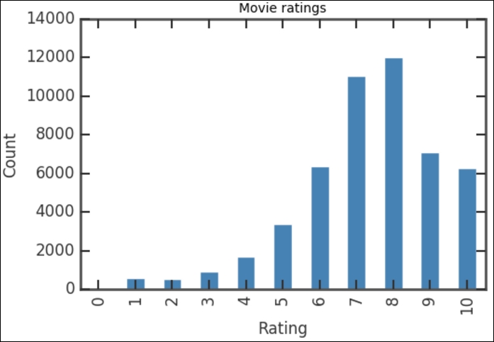
The vertical bars show how many voters that have given a certain rating, covering all the movies in the database. The distribution of the ratings is not very surprising: the counts increase up to a rating of 8, and the count of 9-10 ratings is smaller as most people are reluctant to give the highest rating. If you check the values of the bar for each rating, you can see that it corresponds to what we had previously when printing the rating_counts object. To see what happens if you do not sort the ratings first, plot the rating_counts object, that is, run rating_counts.plot(kind='bar', color='SteelBlue') in a cell.

Let's say that we would like to know if the ratings distribution for a particular movie genre, say Crime Drama, is similar to the overall distribution. We need to cross-reference the ratings information with the movie information, contained in the movies.dat file. To read this file and store it in a Pandas DataFrame object, use the following command:

    cols = ['movie id','movie title','genre']
    movies = pd.read_csv('data/movies.dat', sep='::',
                         index_col=False, names=cols,
                         encoding="UTF-8")

We are again using the read_csv() function to read the data. The column names were obtained from the README.md file distributed with the data. Notice that the separator used in this file is also a double colon, ::. The first few lines of the table can be displayed with the command:

movies[:5]

Notice how the genres are indicated, clumped together with a vertical bar, |, as separator. This is due to the fact that a movie can belong to more than one genre. We can now select only the movies that are crime dramas using the following lines:

drama = movies[movies['genre']=='Crime|Drama']

Notice that this uses the standard indexing notation with square brackets, movies[...]. Instead of specifying a numeric or string index, however, we are using the Boolean movies['genre']=='Crime|Drama' expression as an index. To understand how this works, run the following code in a cell:

is_drama = movies['genre']=='Crime|Drama'
is_drama[:5]

This displays the following output:

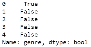
The movies['genre']=='Crime|Drama' expression returns a Series object, where each entry is either True or False, indicating whether the corresponding movie is a crime drama or not, respectively.

Thus, the net effect of the drama = movies[movies['genre']=='Crime|Drama'] assignment is to select all the rows in the movies table for which the entry in the genre column is equal to Crime|Drama and store the result in the drama variable, which is an object of the DataFrame type.

All that we need is the movie id column of this table, which can be selected with the following statement:

drama_ids = drama['movie id']

This, again, uses standard indexing with a string to select a column from a table.

The next step is to extract those entries that correspond to dramas from the ratings table. This requires yet another indexing trick. The code is contained in the following lines:

criterion = ratings['item id'].map(lambda x:(drama_ids==x).any())
drama_ratings = ratings[criterion]

The key to how this code works is the definition of the variable criterion. We want to look up each row of the ratings table and check whether the item id entry is in the drama_ids table. This can be conveniently done by the map() method. This method applies a function to all the entries of a Series object. In our example, the function is as follows:

    lambda x:(drama_ids==x).any()

This function simply checks whether an item appears in drama_ids, and if it does, it returns True. The resulting object criterion will be a Series that contains the True value only in the rows that correspond to dramas. You can view the first rows with the following code:

criterion[:10]

We then use the criterion object as an index to select the rows from the ratings table.

We are now done with selecting the data that we need. To produce a rate count and bar chart, we use the same commands as before. The details are in the following code, which can be run in a single execution cell:

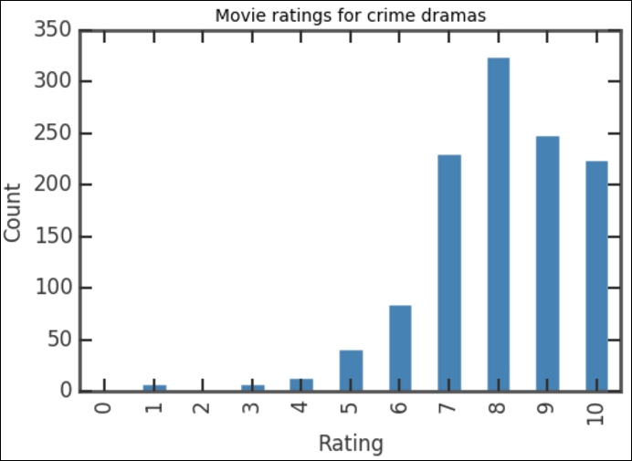
rating_counts = drama_ratings['rating'].value_counts()
sorted_counts = rating_counts.sort_index()
sorted_counts.plot(kind='bar', color='SteelBlue')
plt.title('Movie ratings for dramas')
plt.xlabel('Rating')
plt.ylabel('Count')

As before, this code first computes the counts, indexes them according to the ratings, and then produces a bar chart. This produces a graph that seems to be similar to the overall ratings distribution, as shown in the following figure: