R is an object-oriented language; accordingly, everything in R is an object. Objects belong to classes, with each class characterized by certain properties. The class to which an object belongs to determines the object's properties and the actions we can do with that object. To use an analogy, a gray Mitsubishi Super-Lancer model 1996 object belongs to the class car. It has specific attributes (such as color, model, and manufacturer) for each of the data fields a car object has. It satisfies all criteria that the car class entails; thus, the actions that are applicable to cars (such as igniting the engine and accelerating or using the breaks) are also meaningful with that particular object. In much the same way, a multi-band raster object in R will obligatorily have certain properties (such as the number of rows and columns, and resolution) and applicable actions (such as creating a subset of only the first band or calculating an overlay based on all bands).

All objects that are stored in memory can be accessed using their names, which begin with a character (without quotes; some functions, such as all arithmetic and logical operators can be called using their respective symbol within quotes, such as in "*" as we saw earlier). For example, sqrt is the name of the square root function object; the class to which this object belongs is function. When starting R, a predefined set of objects is loaded into memory, for example, the sqrt function and logical constant values TRUE and FALSE. Another example of a preloaded object is the number :

> pi
[1] 3.141593

The class function returns the class name of the object that it receives as an argument:

> class(TRUE)
[1] "logical"
> class(1)
[1] "numeric"
> class(pi)
[1] "numeric"
> class("a")
[1] "character"
> class(sqrt)
[1] "function"

From the point of view of a typical R user, all objects we handle in R can be divided into two groups: data structures (which hold data) and functions (which are used to perform operations on the data).

The basic components of all data structures are constant values, usually numeric, character, or logical (the last code section shows examples of all three). The simplest data structure in R is a vector, which is covered in Chapter 2, Working with Vectors and Time Series. Later, we'll see how more complex data structures are essentially collections of the simpler data structures. For example, a raster object in R may include two numeric vectors (holding the raster values and its dimensions) and a character vector (holding the Coordinate Reference System (CRS) information). The object-oriented nature of the language makes things easier both for the people who define the data structure classes (since they can build upon predefined simpler classes, rather than starting from the beginning) and for the users (since they can utilize their previous knowledge of the simpler data structure components to quickly understand more complex ones).

Objects of the second type—functions—are typically used to perform operations on data structures. A function may have its influence limited to the R environment, or it may invoke side effects affecting the environment outside of R. All functions we have used until now affect only the R environment; a function to save a raster file, for example, has an external effect—it influences the data content of the hard drive.

Finally, let's take a look at a complete code section that performs a simple spatial analysis operation:

> library(raster)
> r = raster("C:\\Data\\rainfall.tif")
> r[120, 120] = 1000
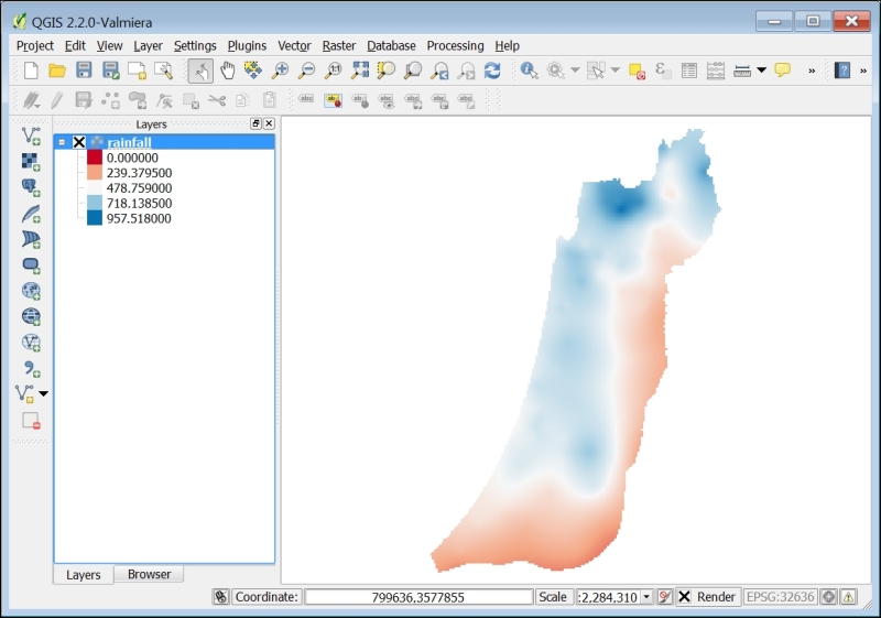
> writeRaster(r, "C:\\Data\\rainfall2.tif")

The task that this code performs is to read a raster file, rainfall.tif, from the disk (look at the following screenshot to see its visualization in QGIS), change one of its values (the one at row 120 line 120, into 1000) and write the resulting raster to a different file.

Do not worry if you do not understand all the lines of code given in the beginning of this section. They will become clear by the time you finish reading Chapter 4, Working with Rasters. Briefly, the first line of code tells R to load the set of functions that are used to work with rasters (called the raster package), such as the raster and writeRaster functions that we use here to read and write raster files. In the second line, we read the requested file and load it into memory. In the third line of code, we assign the value 1000 to the specified pixel of that raster. The fourth line of code writes the new (modified) raster to the disk.

The task indeed sounds simple, but when we use desktop GIS software, it may not be easy to perform through the menus and dialog box system (where direct access to raster values may be unavailable). For example, we may have to create a new point feature over the pixel that we want to change (120,120) in raster A, convert it to a raster B (with the value of 1 at the (120,120) pixel and 0 in all other pixels), and then use an overlay tool to say that we want the pixel in raster A that overlays the value of 1 in raster B to have the value of 1000, while all other pixels retain their original values. Finally, we might need to use an additional toolbox to export the new raster. However, what if we need to perform this operation on several files or repeatedly on a given file as new information comes in?

Generally speaking, when we use programming rather than menu-based interfaces, the steps we have to take may seem less intuitive (writing code rather than scrolling, clicking with the mouse, and filling out dialog boxes). However, we have much more power with giving the computer specific instructions. The beauty of using programming for data analysis, and using R for geospatial analysis in particular, is not only that we gain greater efficiency through automation, but also that we get closer to the data and discover a wide range of new possibilities to analyze it, some of which may not even come to mind when we use a predefined set of tools or menus.