
Here we will be looking at the most useful data structures which exist in R and use using them on some fictional examples to get a better grasp on their syntax and constructs. The main data structures which we will be covering here include:
Vectors
Arrays and matrices
Lists
Data frames
These data structures are used widely inside R as well as by various R packages and functions, including machine learning functions and algorithms which we will be using in the subsequent chapters. So it is essential to know how to use these data structures to work with data efficiently.
Just like we mentioned briefly in the previous sections, vectors are the most basic data type inside R. We use vectors to represent anything, be it input or output. We previously saw how we create vectors and apply mathematical operations on them. We will see some more examples here.
Here we will look at ways to initialize vectors, some of which we had also worked on previously, using operators such as : and functions such as c. In the following code snippet, we will use the seq family of functions to initialize vectors in different ways.
> c(2.5:4.5, 6, 7, c(8, 9, 10), c(12:15))
 [1]  2.5  3.5  4.5  6.0  7.0  8.0  9.0 10.0 12.0 13.0 14.0 15.0
> vector("numeric", 5)
[1] 0 0 0 0 0
> vector("logical", 5)
[1] FALSE FALSE FALSE FALSE FALSE
> logical(5)
[1] FALSE FALSE FALSE FALSE FALSE
> # seq is a function which creates sequences
> seq.int(1,10)
 [1]  1  2  3  4  5  6  7  8  9 10
> seq.int(1,10,2)
[1] 1 3 5 7 9
> seq_len(10)
 [1]  1  2  3  4  5  6  7  8  9 10
One of the most important operations we can do on vectors involves subsetting and indexing vectors to access specific elements which are often useful when we want to run some code only on specific data points. The following examples show some ways in which we can index and subset vectors:
> vec <- c("R", "Python", "Julia", "Haskell", "Java", "Scala")
> vec[1]
[1] "R"
> vec[2:4]
[1] "Python"  "Julia"   "Haskell"
> vec[c(1, 3, 5)]
[1] "R"     "Julia" "Java"
> nums <- c(5, 8, 10, NA, 3, 11)
> nums
[1]  5  8 10 NA  3 11
> which.min(nums)   # index of the minimum element
[1] 5
> which.max(nums)   # index of the maximum element
[1] 6
> nums[which.min(nums)]  # the actual minimum element
[1] 3
> nums[which.max(nums)]  # the actual maximum element
[1] 11
Now we look at how we can name vectors. This is basically a nifty feature in R where you can label each element in a vector to make it more readable or easy to interpret. There are two ways this can be done, which are shown in the following examples:
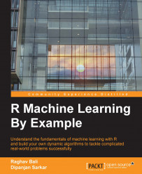
> c(first=1, second=2, third=3, fourth=4, fifth=5)
Output:
> positions <- c(1, 2, 3, 4, 5)
> names(positions)
NULL
> names(positions) <- c("first", "second", "third", "fourth", "fifth")
> positions
Output:
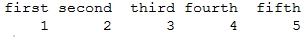
> names(positions)
[1] "first"  "second" "third"  "fourth" "fifth"
> positions[c("second", "fourth")]
Output:
Thus, you can see, it becomes really useful to annotate and name vectors sometimes, and we can also subset and slice vectors using element names rather than values.
Vectors are one dimensional data structures, which means that they just have one dimension and we can get the number of elements they have using the length property. Do remember that arrays may also have a similar meaning in other programming languages, but in R they have a slightly different meaning. Basically, arrays in R are data structures which hold the data having multiple dimensions. Matrices are just a special case of generic arrays having two dimensions, namely represented by properties rows and columns. Let us look at some examples in the following code snippets in the accompanying subsection.
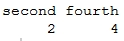
First we will create an array that has three dimensions. Now it is easy to represent two dimensions in your screen, but to go one dimension higher, there are special ways in which R transforms the data. The following example shows how R fills the data (column first) in each dimension and shows the final output for a 4x3x3 array:
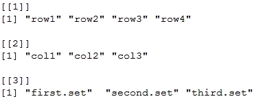
> three.dim.array <- array(
+     1:32,    # input data
+     dim = c(4, 3, 3),   # dimensions
+     dimnames = list(    # names of dimensions
+         c("row1", "row2", "row3", "row4"),
+         c("col1", "col2", "col3"),
+         c("first.set", "second.set", "third.set")
+     )
+ )
> three.dim.array
Output:
Like I mentioned earlier, a matrix is just a special case of an array. We can create a matrix using the matrix function, shown in detail in the following example. Do note that we use the parameter byrow to fill the data row-wise in the matrix instead of R's default column-wise fill in any array or matrix. The ncol and nrow parameters stand for number of columns and rows respectively.
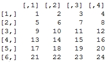
> mat <- matrix(
+     1:24,   # data
+     nrow = 6,  # num of rows
+     ncol = 4,  # num of columns
+     byrow = TRUE,  # fill the elements row-wise
+ )
> mat
Output:
Just like we named vectors and accessed element names, will perform similar operations in the following code snippets. You have already seen the use of the dimnames parameter in the preceding examples. Let us look at some more examples as follows:
> dimnames(three.dim.array)
Output:
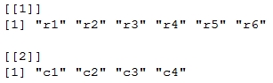
> rownames(three.dim.array)
[1] "row1" "row2" "row3" "row4"
> colnames(three.dim.array)
[1] "col1" "col2" "col3"
> dimnames(mat)
NULL
> rownames(mat)
NULL
> rownames(mat) <- c("r1", "r2", "r3", "r4", "r5", "r6")
> colnames(mat) <- c("c1", "c2", "c3", "c4")
> dimnames(mat)
Output:
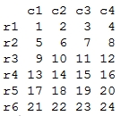
> mat
Output:
To access details of dimensions related to arrays and matrices, there are special functions. The following examples show the same:
> dim(three.dim.array)
[1] 4 3 3
> nrow(three.dim.array)
[1] 4
> ncol(three.dim.array)
[1] 3
> length(three.dim.array)  # product of dimensions
[1] 36
> dim(mat)
[1] 6 4
> nrow(mat)
[1] 6
> ncol(mat)
[1] 4
> length(mat)
[1] 24
A lot of machine learning and optimization algorithms deal with matrices as their input data. In the following section, we will look at some examples of the most common operations on matrices.
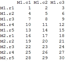
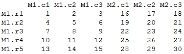
We start by initializing two matrices and then look at ways of combining the two matrices using functions such as c which returns a vector, rbind which combines the matrices by rows, and cbind which does the same by columns.
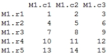
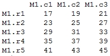
> mat1 <- matrix(
+     1:15,
+     nrow = 5,
+     ncol = 3,
+     byrow = TRUE,
+     dimnames = list(
+         c("M1.r1", "M1.r2", "M1.r3", "M1.r4", "M1.r5")
+         ,c("M1.c1", "M1.c2", "M1.c3")
+     )
+ )
> mat1
Output:
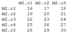
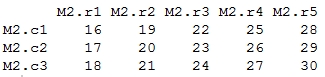
> mat2 <- matrix(
+     16:30,
+     nrow = 5,
+     ncol = 3,
+     byrow = TRUE,
+     dimnames = list(
+         c("M2.r1", "M2.r2", "M2.r3", "M2.r4", "M2.r5"),
+         c("M2.c1", "M2.c2", "M2.c3")
+     )
+ )
> mat2
Output:
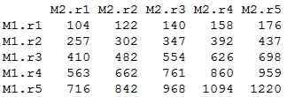
> rbind(mat1, mat2)
Output:
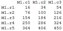
> cbind(mat1, mat2)
Output:
> c(mat1, mat2)
Output:

Now we look at some of the important arithmetic operations which can be performed on matrices. Most of them are quite self-explanatory from the following syntax:
> mat1 + mat2 # matrix addition
Output:
> mat1 * mat2 # element-wise multiplication
Output:
> tmat2 <- t(mat2)  # transpose
> tmat2
Output:
> mat1 %*% tmat2 # matrix inner product
Output:
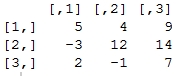
> m <- matrix(c(5, -3, 2, 4, 12, -1, 9, 14, 7), nrow = 3, ncol = 3)
> m
Output:
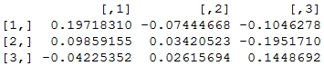
> inv.m <- solve(m)  # matrix inverse
> inv.m
Output:
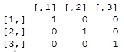
> round(m %*% inv.m) # matrix * matrix_inverse = identity matrix
Output:
The preceding arithmetic operations are just some of the most popular ones amongst the vast number of functions and operators which can be applied to matrices. This becomes useful, especially in areas such as linear optimization.
Lists are a special case of vectors where each element in the vector can be of a different type of data structure or even simple data types. It is similar to the lists in the Python programming language in some aspects, if you have used it before, where the lists indicate elements which can be of different types and each have a specific index in the list. In R, each element of a list can be as simple as a single element or as complex as a whole matrix, a function, or even a vector of strings.
We will get started with looking at some common methods to create and initialize lists in the following examples. Besides that, we will also look at how we can access some of these list elements for further computations. Do remember that each element in a list can be a simple primitive data type or even complex data structures or functions.
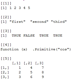
> list.sample <- list(
+     1:5,

+     c("first", "second", "third"),
+     c(TRUE, FALSE, TRUE, TRUE),
+     cos,
+     matrix(1:9, nrow = 3, ncol = 3)
+ )
> list.sample
Output:
> list.with.names <- list(
+     even.nums = seq.int(2,10,2),
+     odd.nums  = seq.int(1,10,2),
+     languages = c("R", "Python", "Julia", "Java"),
+     cosine.func = cos
+ )
> list.with.names
Output:
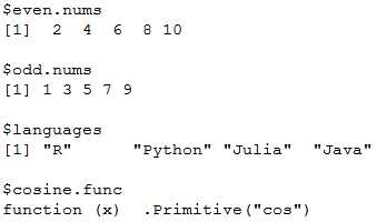
> list.with.names$cosine.func
function (x)  .Primitive("cos")
> list.with.names$cosine.func(pi)
[1] -1
>
> list.sample[[4]]
function (x)  .Primitive("cos")
> list.sample[[4]](pi)
[1] -1
>
> list.with.names$odd.nums
[1] 1 3 5 7 9
> list.sample[[1]]
[1] 1 2 3 4 5
> list.sample[[3]]
[1]  TRUE FALSE  TRUE  TRUE
You can see from the preceding examples how easy it is to access any element of the list and use it for further computations, such as the cos function.
Now we will take a look at how to combine several lists together into one single list in the following examples:
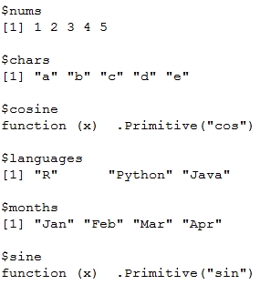
> l1 <- list(
+     nums = 1:5,
+     chars = c("a", "b", "c", "d", "e"),
+     cosine = cos
+ )
> l2 <- list(
+     languages = c("R", "Python", "Java"),
+     months = c("Jan", "Feb", "Mar", "Apr"),
+     sine = sin
+ )
> # combining the lists now
> l3 <- c(l1, l2)
> l3
Output:
It is very easy to convert lists in to vectors and vice versa. The following examples show some common ways we can achieve this:
> l1 <- 1:5
> class(l1)
[1] "integer"
> list.l1 <- as.list(l1)
> class(list.l1)
[1] "list"
> list.l1
Output:
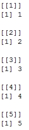
> unlist(list.l1)
[1] 1 2 3 4 5
Data frames are special data structures which are typically used for storing data tables or data in the form of spreadsheets, where each column indicates a specific attribute or field and the rows consist of specific values for those columns. This data structure is extremely useful in working with datasets which usually have a lot of fields and attributes.
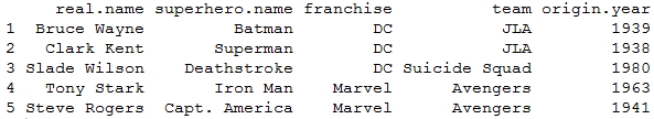
We can create data frames easily using the data.frame function. We will look at some following examples to illustrate the same with some popular superheroes:
> df <- data.frame(
+     real.name = c("Bruce Wayne", "Clark Kent", "Slade Wilson", "Tony Stark", "Steve Rogers"),
+     superhero.name = c("Batman", "Superman", "Deathstroke", "Iron Man", "Capt. America"),
+     franchise = c("DC", "DC", "DC", "Marvel", "Marvel"),
+     team = c("JLA", "JLA", "Suicide Squad", "Avengers", "Avengers"),
+     origin.year = c(1939, 1938, 1980, 1963, 1941)
+ )
> df
Output:
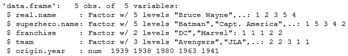
> class(df)
[1] "data.frame"
> str(df)
Output:
> rownames(df)
[1] "1" "2" "3" "4" "5"
> colnames(df)
Output:

> dim(df)
[1] 5 5
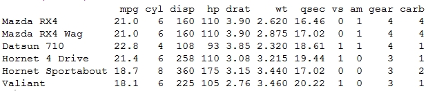
The str function talks in detail about the structure of the data frame where we see details about the data present in each column of the data frame. There are a lot of datasets readily available in R base which you can directly load and start using. One of them is shown next. The mtcars dataset has information about various automobiles, which was extracted from the Motor Trend U.S. Magazine of 1974.
> head(mtcars) # one of the datasets readily available in R
Output:
There are a lot of operations we can do on data frames, such as merging, combining, slicing, and transposing data frames. We will look at some of the important data frame operations in the following examples.
It is really easy to index and subset specific data inside data frames using simplex indexes and functions such as subset.
> df[2:4,]
Output:
> df[2:4, 1:2]
Output:
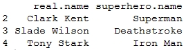
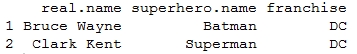
> subset(df, team=="JLA", c(real.name, superhero.name, franchise))
Output:
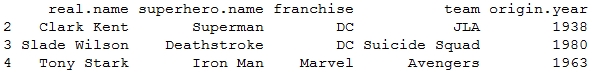
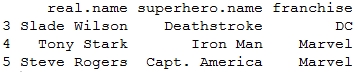
> subset(df, team %in% c("Avengers","Suicide Squad"), c(real.name, superhero.name, franchise))
Output:
We will now look at some more complex operations, such as combining and merging data frames.
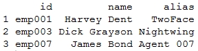
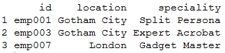
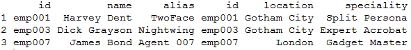
> df1 <- data.frame(
+     id = c('emp001', 'emp003', 'emp007'),
+     name = c('Harvey Dent', 'Dick Grayson', 'James Bond'),
+     alias = c('TwoFace', 'Nightwing', 'Agent 007')
+ )
>
> df2 <- data.frame(
+     id = c('emp001', 'emp003', 'emp007'),
+     location = c('Gotham City', 'Gotham City', 'London'),
+     speciality = c('Split Persona', 'Expert Acrobat', 'Gadget Master')
+ )
> df1
Output:
> df2
Output:
> rbind(df1, df2)   # not possible since column names don't match
Error in match.names(clabs, names(xi)) :
  names do not match previous names
> cbind(df1, df2)
Output:
> merge(df1, df2, by="id")
Output:
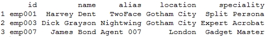
From the preceding operations it is evident that rbind and cbind work in the same way as we saw previously with arrays and matrices. However, merge lets you merge the data frames in the same way as you join various tables in relational databases.