

When we start to use neural networks, we will use activation functions regularly because activation functions are a mandatory part of any neural network. The goal of the activation function is to adjust weight and bias. In TensorFlow, activation functions are non-linear operations that act on tensors. They are functions that operate in a similar way to the previous mathematical operations. Activation functions serve many purposes, but a few main concepts is that they introduce a non-linearity into the graph while normalizing the outputs. Start a TensorFlow graph with the following commands:
import tensorflow as tf
sess = tf.Session()
The activation functions live in the neural network (nn) library in TensorFlow. Besides using built-in activation functions, we can also design our own using TensorFlow operations. We can import the predefined activation functions (import tensorflow.nn as nn) or be explicit and write .nn in our function calls. Here, we choose to be explicit with each function call:
The rectified linear unit, known as ReLU, is the most common and basic way to introduce a non-linearity into neural networks. This function is just
max(0,x). It is continuous but not smooth. It appears as follows:print(sess.run(tf.nn.relu([-3., 3., 10.]))) [ 0. 3. 10.]
There will be times when we wish to cap the linearly increasing part of the preceding ReLU activation function. We can do this by nesting the
max(0,x)function into amin()function. The implementation that TensorFlow has is called the ReLU6 function. This is defined asmin(max(0,x),6). This is a version of the hard-sigmoid function and is computationally faster, and does not suffer from vanishing (infinitesimally near zero) or exploding values. This will come in handy when we discuss deeper neural networks in Chapters 8, Convolutional Neural Networks and Chapter 9, Recurrent Neural Networks. It appears as follows:print(sess.run(tf.nn.relu6([-3., 3., 10.]))) [ 0. 3. 6.]
The sigmoid function is the most common continuous and smooth activation function. It is also called a logistic function and has the form 1/(1+exp(-x)). The sigmoid is not often used because of the tendency to zero-out the back propagation terms during training. It appears as follows:
print(sess.run(tf.nn.sigmoid([-1., 0., 1.])))
[ 0.26894143  0.5         0.7310586 ]
Another smooth activation function is the hyper tangent. The hyper tangent function is very similar to the sigmoid except that instead of having a range between
0and1, it has a range between-1and1. The function has the form of the ratio of the hyperbolic sine over the hyperbolic cosine. But another way to write this is ((exp(x)-exp(-x))/(exp(x)+exp(-x)). It appears as follows:print(sess.run(tf.nn.tanh([-1., 0., 1.]))) [-0.76159418 0. 0.76159418 ]
The
softsignfunction also gets used as an activation function. The form of this function is x/(abs(x) + 1). Thesoftsignfunction is supposed to be a continuous approximation to the sign function. It appears as follows:print(sess.run(tf.nn.softsign([-1., 0., -1.]))) [-0.5 0. 0.5]
Another function, the
softplus, is a smooth version of the ReLU function. The form of this function is log(exp(x) + 1). It appears as follows:print(sess.run(tf.nn.softplus([-1., 0., -1.]))) [ 0.31326166 0.69314718 1.31326163]
The Exponential Linear Unit (ELU) is very similar to the
softplusfunction except that the bottom asymptote is-1instead of0. The form is (exp(x)+1) if x < 0 else x. It appears as follows:print(sess.run(tf.nn.elu([-1., 0., -1.]))) [-0.63212055 0. 1. ]
These activation functions are the way that we introduce nonlinearities in neural networks or other computational graphs in the future. It is important to note where in our network we are using activation functions. If the activation function has a range between 0 and 1 (sigmoid), then the computational graph can only output values between 0 and 1.
If the activation functions are inside and hidden between nodes, then we want to be aware of the effect that the range can have on our tensors as we pass them through. If our tensors were scaled to have a mean of zero, we will want to use an activation function that preserves as much variance as possible around zero. This would imply we want to choose an activation function such as the hyperbolic tangent (tanh) or softsign. If the tensors are all scaled to be positive, then we would ideally choose an activation function that preserves variance in the positive domain.
Here are two graphs that illustrate the different activation functions. The following figure shows the following functions ReLU, ReLU6, softplus, exponential LU, sigmoid, softsign, and the hyperbolic tangent:
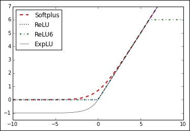
Figure 3: Activation functions of softplus, ReLU, ReLU6, and exponential LU
In Figure 3, we can see four of the activation functions, softplus, ReLU, ReLU6, and exponential LU. These functions flatten out to the left of zero and linearly increase to the right of zero, with the exception of ReLU6, which has a maximum value of 6:
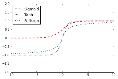
Figure 4: Sigmoid, hyperbolic tangent (tanh), and softsign activation function
In Figure 4, we have the activation functions sigmoid, hyperbolic tangent (tanh), and softsign. These activation functions are all smooth and have a S n shape. Note that there are two horizontal asymptotes for these functions.