
This section is the most important one. Here, we will try a couple of different ML algorithms in order to get an idea about which ML algorithm performs better. Also, we will perform a training accuracy comparison.
By this time, you will definitely know that this particular problem is considered a classification problem. The algorithms that we are going to choose are as follows (this selection is based on intuition):
K-Nearest Neighbor (KNN)
Logistic Regression
AdaBoost
GradientBoosting
RandomForest
Our first step is to generate the training data in a certain format. We are going to split the training dataset into a training and testing dataset. So, basically, we are preparing the input for our training. This is common for all the ML algorithms. Refer to the code snippet in the following figure:
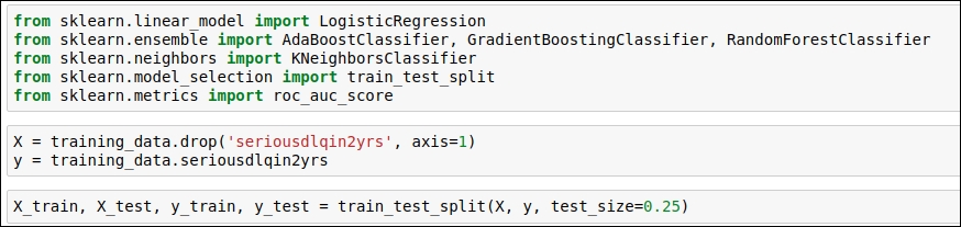
Figure 1.46: Code snippet for generating a training dataset in the key-value format for training
As you can see in the code, variable x contains all the columns except the target column entitled seriousdlqin2yrs, so we have dropped this column. The reason behind dropping this attribute is that this attribute contains the answer/target/label for each row. ML algorithms need input in terms of a key-value pair, so a target column is key and all other columns are values. We can say that a certain pattern of values will lead to a particular target value, which we need to predict using an ML algorithm.
Here, we also split the training data. We will use 75% of the training data for actual training purposes, and once training is completed, we will use the remaining 25% of the training data to check the training accuracy of our trained ML model. So, without wasting any time, we will jump to the coding of the ML algorithms, and I will explain the code to you as and when we move forward. Note that here, I'm not get into the mathematical explanation of the each ML algorithm but I am going to explain the code.
In this algorithm, generally, our output prediction follows the same tendency as that of its neighbor. K is the number of neighbors that we are going to consider. If K=3, then during the prediction output, check the three nearest neighbor points, and if one neighbor belongs to X category and two neighbors belongs to Y category, then the predicted label will be Y, as the majority of the nearest points belongs to the Y category.
Let's see what we have coded. Refer to the following figure:

Figure 1.47: Code snippet for defining the KNN classifier
Let's understand the parameters one by one:
As per the code, K=5 means our prediction is based on the five nearest neighbors. Here,
n_neighbors=5.Weights are selected uniformly, which means all the points in each neighborhood are weighted equally. Here, weights='uniform'.
algorithm='auto': This parameter will try to decide the most appropriate algorithm based on the values we passed.
leaf_size = 30: This parameter affects the speed of the construction of the model and query. Here, we have used the default value, which is 30.
p=2: This indicates the power parameter for the Minkowski metric. Here, p=2 uses
euclidean_distance.metric='minkowski': This is the default distance metric, which helps us build the tree.
metric_params=None: This is the default value that we are using.
Logistic regression is one of most widely used ML algorithms and is also one of the oldest. This algorithm generates probability for the target variable using sigmod and other nonlinear functions in order to predict the target labels.
Let's refer to the code and the parameter that we have used for Logistic regression. You can refer to the code snippet given in the following figure:
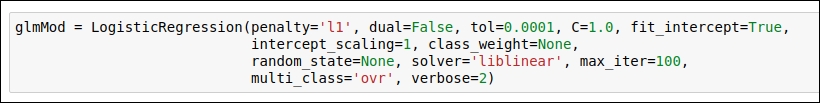
Figure 1.48: Code snippet for the Logistic regression ML algorithm
Let's understand the parameters one by one:
penalty='l1': This parameter indicates the choice of the gradient descent algorithm. Here, we have selected the Newton-Conjugate_Gradient method.
dual=False: If we have number of sample > number of features, then we should set this parameter as false.
tol=0.0001: This is one of the stopping criteria for the algorithm.
c=1.0: This value indicates the inverse of the regularization strength. This parameter must be a positive float value.
fit_intercept = True: This is a default value for this algorithm. This parameter is used to indicate the bias for the algorithm.
solver='liblinear': This algorithm performs well for small datasets, so we chose that.
intercept_scaling=1: If we select the liblinear algorithm and fit_intercept = True, then this parameter helps us generate the feature weight.
class_weight=None: There is no weight associated with the class labels.
random_state=None: Here, we use the default value of this parameter.
max_iter=100: Here, we iterate 100 times in order to converge our ML algorithm on the given dataset.
multi_class='ovr': This parameter indicates that the given problem is the binary classification problem.
verbose=2: If we use the liblinear in the solver parameter, then we need to put in a positive number for verbosity.
The AdaBoost algorithm stands for Adaptive Boosting. Boosting is an ensemble method in which we will build strong classifier by using multiple weak classifiers. AdaBoost is boosting algorithm giving good result for binary classification problems. If you want to learn more about it then refer this article https://machinelearningmastery.com/boosting-and-adaboost-for-machine-learning/.
This particular algorithm has N number of iterations. In the first iteration, we start by taking random data points from the training dataset and building the model. After each iteration, the algorithm checks for data points in which the classifier doesn't perform well. Once those data points are identified by the algorithm based on the error rate, the weight distribution is updated. So, in the next iteration, there are more chances that the algorithm will select the previously poorly classified data points and learn how to classify them. This process keeps running for the given number of iterations you provide.
Let's refer to the code snippet given in the following figure:

Figure 1.49: Code snippet for the AdaBosst classifier
The parameter-related description is given as follows:
base_estimator = None: The base estimator from which the boosted ensemble is built.
n_estimators=200: The maximum number of estimators at which boosting is terminated. After 200 iterations, the algorithm will be terminated.
learning_rate=1.0: This rate decides how fast our model will converge.
This algorithm is also a part of the ensemble of ML algorithms. In this algorithm, we use basic regression algorithm to train the model. After training, we will calculate the error rate as well as find the data points for which the algorithm does not perform well, and in the next iteration, we will take the data points that introduced the error and retrain the model for better prediction. The algorithm uses the already generated model as well as a newly generated model to predict the values for the data points.
You can see the code snippet in the following figure:

Figure 1.50: Code snippet for the Gradient Boosting classifier
Let's go through the parameters of the classifier:
loss='deviance': This means that we are using logistic regression for classification with probabilistic output.
learning_rate = 0.1: This parameter tells us how fast the model needs to converge.
n_estimators = 200: This parameter indicates the number of boosting stages that are needed to be performed.
subsample = 1.0: This parameter helps tune the value for bias and variance. Choosing subsample < 1.0 leads to a reduction in variance and an increase in bias.
min_sample_split=2: The minimum number of samples required to split an internal node.
min_weight_fraction_leaf=0.0: Samples have equal weight, so we have provided the value 0.
max_depth=3: This indicates the maximum depth of the individual regression estimators. The maximum depth limits the number of nodes in the tree.
init=None: For this parameter, loss.init_estimator is used for the initial prediction.
random_state=None: This parameter indicates that the random state is generated using the
numpy.randomfunction.max_features=None: This parameter indicates that we have N number of features. So,
max_features=n_features.verbose=0: No progress has been printed.
This particular ML algorithm generates the number of decision trees and uses the voting mechanism to predict the target label. In this algorithm, there are a number of decision trees generated, creating a forest of trees, so it's called RandomForest.
In the following code snippet, note how we have declared the RandomForest classifier:
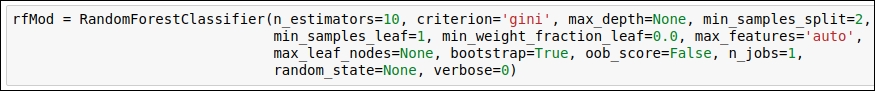
Figure 1.51: Code snippet for Random Forest Classifier
Let's understand the parameters here:
n_estimators=10: This indicates the number of trees in the forest.criterion='gini': Information gained will be calculated by gini.max_depth=None: This parameter indicates that nodes are expanded until all leaves are pure or until all leaves contain less than min_samples_split samples.min_samples_split=2: This parameter indicates that there is a minimum of two samples required to perform splitting in order to generate the tree.min_samples_leaf=1: This indicates the sample size of the leaf node.min_weight_fraction_leaf=0.0: This parameter indicates the minimum weighted fraction of the sum total of weights (of all the input samples) required to be at a leaf node. Here, weight is equally distributed, so a sample weight is zero.max_features='auto': This parameter is considered using the auto strategy. We select the auto value, and then we select max_features=sqrt(n_features).max_leaf_nodes=None: This parameter indicates that there can be an unlimited number of leaf nodes.bootstrap=True: This parameter indicates that the bootstrap samples are used when trees are being built.oob_score=False: This parameter indicates whether to use out-of-the-bag samples to estimate the generalization accuracy. We are not considering out-of-the-bag samples here.n_jobs=1: Both fit and predict job can be run in parallel ifn_job = 1.random_state=None: This parameter indicates that random state is generated using thenumpy.randomfunction.verbose=0: This controls the verbosity of the tree building process. 0 means we are not printing the progress.
Up until now, we have seen how we declare our ML algorithm. We have also defined some parameter values. Now, it's time to train this ML algorithm on the training dataset. So let's discuss that.