

In this section, we will look at some of the widely used testing matrices that we can use in order to get an idea about how good or bad our trained model is. This testing score gives us a fair idea about which model achieves the highest accuracy when it comes to the prediction of the 25% of the data.
Here, we are using two basic levels of the testing matrix:
The mean accuracy of the trained models
The ROC-AUC score
In this section, we will understand how scikit-learn calculates the accuracy score when we use the scikit-learn function score() to generate the training accuracy. The function score() returns the mean accuracy. More precisely, it uses residual standard error. Residual standard error is nothing but the positive square root of the mean square error. Here, the equation for calculating accuracy is as follows:
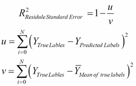
The best possible score is 1.0 and the model can have a negative score as well (because the model can be arbitrarily worse). If a constant model always predicts the expected value of y, disregarding the input features, it will get a residual standard error score of 0.0.
The ROC-AUC score is used to find out the accuracy of the classifier. ROC and AUC are two different terms. Let's understand each of the terms one by one.
ROC stands for Receiver Operating Characteristic. It's is a type of curve. We draw the ROC curve to visualize the performance of the binary classifier. Now that I have mentioned that ROC is a curve, you may want to know which type of curve it is, right? The ROC curve is a 2-D curve. It's x axis represents the False Positive Rate (FPR) and its y axis represents the True Positive Rate (TPR). TPR is also known as sensitivity, and FPR is also known as specificity (SPC). You can refer to the following equations for FPR and TPR.
TPR = True Positive / Number of positive samples = TP / P
FPR = False Positive / Number of negative samples = FP / N = 1 - SPC
For any binary classifier, if the predicted probability is ≥ 0.5, then it will get the class label X, and if the predicted probability is < 0.5, then it will get the class label Y. This happens by default in most binary classifiers. This cut-off value of the predicted probability is called the threshold value for predictions. For all possible threshold values, FPR and TPR have been calculated. This FPR and TPR is an x,y value pair for us. So, for all possible threshold values, we get the x,y value pairs, and when we put the points on an ROC graph, it will generate the ROC curve. If your classifier perfectly separates the two classes, then the ROC curve will hug the upper-right corner of the graph. If the classifier performance is based on some randomness, then the ROC curve will align more to the diagonal of the ROC curve. Refer to the following figure:
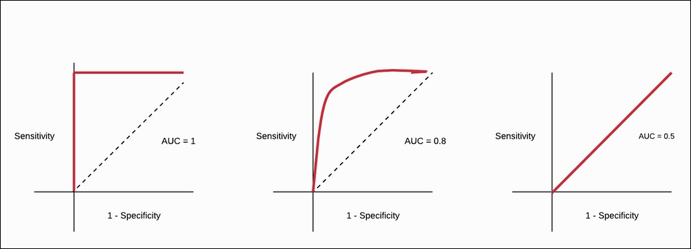
Figure 1.53: ROC curve for different classification scores
In the preceding figure, the leftmost ROC curve is for the perfect classifier. The graph in the center shows the classifier with better accuracy in real-world problems. The classifier that is very random in its guess is shown in the rightmost graph. When we draw an ROC curve, how can we quantify it? In order to answer that question, we will introduce AUC.
AUC stands for Area Under the Curve. In order to quantify the ROC curve, we use the AUC. Here, we will see how much area has been covered by the ROC curve. If we obtain a perfect classifier, then the AUC score is 1.0, and if we have a classifier that is random in its guesses, then the AUC score is 0.5. In the real world, we don't expect an AUC score of 1.0, but if the AUC score for the classifier is in the range of 0.6 to 0.9, then it will be considered a good classifier. You can refer to the following figure:
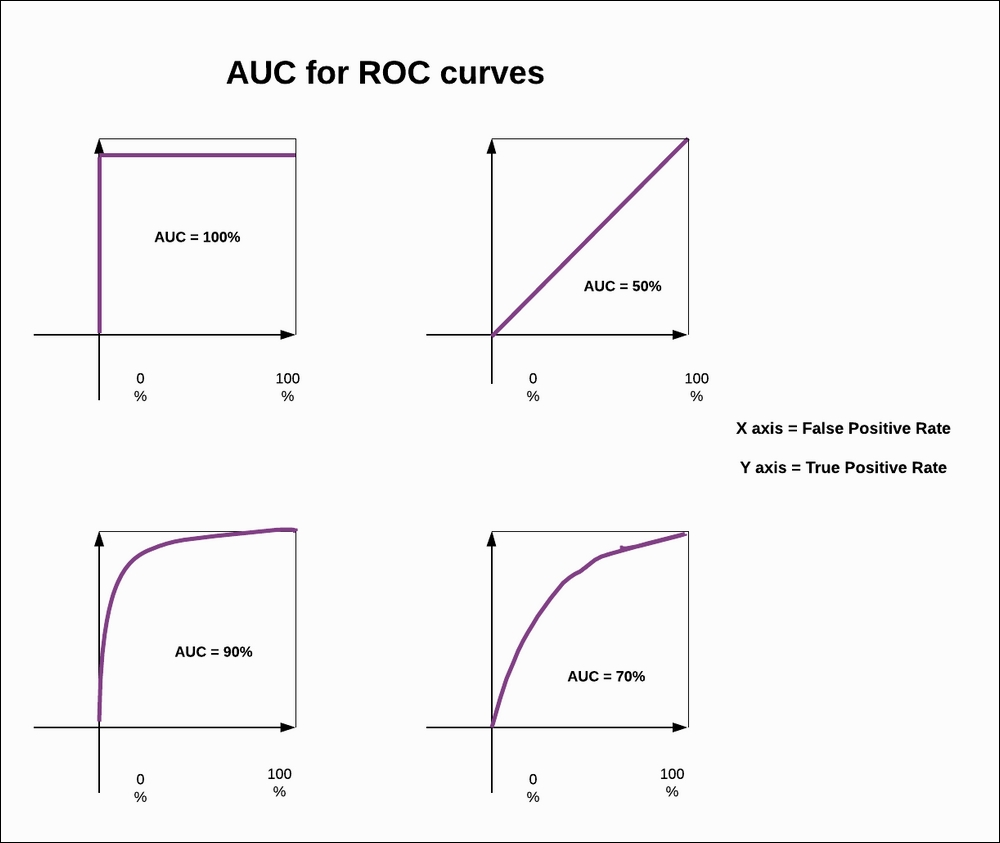
Figure 1.54: AUC for the ROC curve
In the preceding figure, you can see how much area under the curve has been covered, and that becomes our AUC score. This gives us an indication of how good or bad our classifier is performing.
These are the two matrices that we are going to use. In the next section, we will implement actual testing of the code and see the testing matrix for our trained ML models.