
The previous section highlights the different forms of variables. The variables such as Gender, Car_Model, and Minor_Problems possibly take one of the finite values. These variables are particular cases of the more general class of discrete variables.
It is to be noted that the sample space  of a discrete variable need not be finite. As an example, the number of errors on a page may take values on the set of positive integers, {0, 1, 2, …}. Suppose that a discrete random variable X can take values among
  with respective probabilities
  , that is,
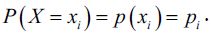 . Then, we require that the probabilities be non-zero and further that their sum be 1:
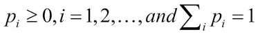
where the Greek symbol  represents summation over the index i.
The function  is called the probability mass function (pmf) of the discrete RV X. We will now consider formal definitions of important families of discrete variables. The engineers may refer to Bury (1999) for a detailed collection of useful statistical distributions in their field. The two most important parameters of a probability distribution are specified by mean and variance of the RV X.
In some cases, and important too, these parameters may not exist for the RV. However, we will not focus on such distributions, though we caution the reader that this does not mean that such RVs are irrelevant. Let us define these parameters for the discrete RV. The mean and variance of a discrete RV are respectively calculated as:
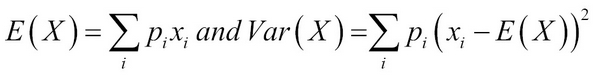
The mean is a measure of central tendency, whereas the variance gives a measure of the spread of the RV.
The variables defined so far are more commonly known as categorical variables. Agresti (2002) defines a categorical variable as a measurement scale consisting of a set of categories.
Let us identify the categories for the variables listed in the previous section. The categories for the Gender variable are male and female; whereas the car category variables derived from Car_Model are hatchback, sedan, station wagon, and utility vehicles. The Minor_Problems and Major_Problems variables have common but independent categories, yes and no; and, finally, the Satisfaction_Rating variable has the categories, as seen earlier, Very Poor, Poor, Average, Good, and Very Good. The Car_Model variable is just a set of labels of the name of car and it is an example of a nominal variable.
Finally, the output of the Satistifaction_Rating variable has an implicit order in it: Very Poor < Poor < Average < Good < Very Good. It may be apparent that this difference poses subtle challenges in their analysis. These types of variables are called ordinal variables. We will look at another type of categorical variable that has not popped up thus far.
Practically, it is often the case that the output of a continuous variable is put in a certain bin for ease of conceptualization. A very popular example is the categorization of the income level or age. In the case of income variables, it has become apparent in one of the earlier studies that people are very conservative about revealing their income in precise numbers.
For example, the author may be shy to reveal that his monthly income is Rs. 34,892. On the other hand, it has been revealed that these very same people do not have a problem in disclosing their income as belonging to one of the following categories: < Rs. 10,000, Rs. 10,000-30,000, Rs. 30,000-50,000, and > Rs. 50,000. Thus, this information may also be coded into labels and then each of the labels may refer to any one value in an interval bin. Thus, such variables are referred as interval variables.
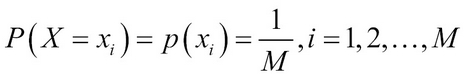
A random variable X is said to be a discrete uniform random variable if it can take any one of the finite M labels with equal probability.
As the discrete uniform random variable X can assume one of the 1, 2, …, M with equal probability, this probability is actually  . As the probability remains the same across the labels, the nomenclature uniform is justified. It might appear at the outset that this is not a very useful random variable. However, the reader is cautioned that this intuition is not correct. As a simple case, this variable arises in many cases where simple random sampling is needed in action. The pmf of a discrete RV is calculated as:
A simple plot of the probability distribution of a discrete uniform RV is demonstrated next:
> M = 10
> mylabels=1:M
> prob_labels=rep(1/M,length(mylabels))
> dotchart(prob_labels,labels=mylabels,xlim=c(.08,.12),
+ xlab=”Probability”)
> title("A Dot Chart for Probability of Discrete Uniform RV”)
Note
Downloading the example code
You can download the example code files for all Packt books you have purchased from your account at http://www.packtpub.com. If you purchased this book elsewhere, you can visit http://www.packtpub.com/support and register to have the files emailed directly to you.
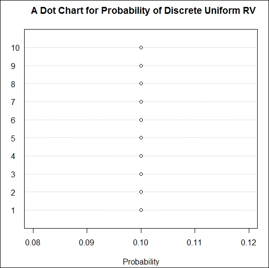
Probability distribution of a discrete uniform random variable
Note
The R programs here are indicative and it is not absolutely necessary that you follow them here. The R programs will actually begin from the next chapter and your flow won’t be affected if you do not understand certain aspects of them.
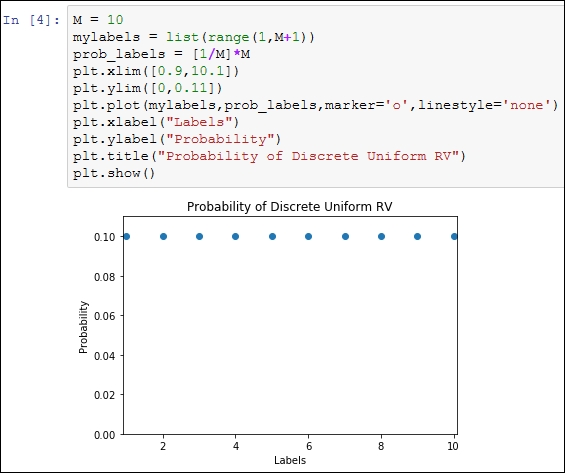
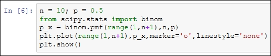
An equivalent Python program and its output is given in the following screenshot:
Recall the second question in the Experiments with uncertainty in computer science section, which asks: How many machines are likely to break down after a period of 1 year, 2 years, and 3 years?. When the outcomes involve uncertainty, the more appropriate question that we ask is related to the probability of the number of break downs being x.
Consider a fixed time frame, say 2 years. To make the question more generic, we assume that we have n number of machines. Suppose that the probability of a breakdown for a given machine at any given time is p. The goal is to obtain the probability of x machines with the breakdown, and implicitly (n-x) functional machines. Now consider a fixed pattern where the first x units have failed and the remaining are functioning properly. All the n machines function independently of other machines. Thus, the probability of observing x machines in the breakdown state is  .
.
Similarly, each of the remaining (n-x) machines have the probability of (1-p) of being in the functional state, and thus the probability of these occurring together is  . Again, by the independence axiom value, the probability of x machines with a breakdown is then given by
  . Finally, in the overall setup, the number of possible samples with a breakdown being x and (n-x) samples being functional is actually the number of possible combinations of choosing x-out-of-n items, which is the combinatorial
  .
.
As each of these samples is equally likely to occur, the probability of exactly x broken machines is given by 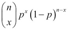 . The RV X obtained in such a context is known as the binomial RV and its pmf is called as the binomial distribution. In mathematical terms, the pmf of the binomial RV is calculated as:
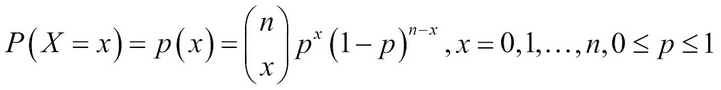
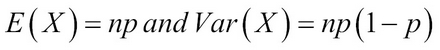
The pmf of a binomial distribution is sometimes denoted by  . Let us now look at some important properties of a binomial RV. The mean and variance of a binomial RV X are respectively calculated as:
Note
As p is always a number between 0 and 1, the variance of a binomial RV is always lesser than its mean.
Example 1.3.1: Suppose n = 10 and p = 0.5. We need to obtain the probabilities p(x), x=0, 1, 2, …, 10. The probabilities can be obtained using the built-in R function, dbinom. The function dbinom returns the probabilities of a binomial RV.
The first argument of this function may be a scalar or a vector according to the points at which we wish to know the probability. The second argument of the function needs to know the value of n, the size of the binomial distribution. The third argument of this function requires the user to specify the probability of success in p. It is natural to forget the syntax of functions and the R help system becomes very handy here. For any function, you can get details of it using ? followed by the function name. Please do not insert a space between ? and the function name. Here, you can try ?dbinom:
> n <- 10; p <- 0.5
> p_x <- round(dbinom(x=0:10, n, p),4)
> plot(x=0:10,p_x,xlab=”x”, ylab=”P(X=x)”)
The R function round fixes the accuracy of the argument up to the specified number of digits.
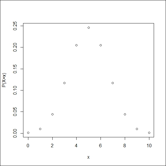
Binomial probabilities
We have used the dbinom function in the previous example. There are three utility facets for the binomial distribution. The three facets are p, q, and r. These three facets respectively help us in computations related to cumulative probabilities, quantiles of the distribution, and simulation of random numbers from the distribution. To use these functions, we simply augment the letters with the distribution name, binom, here, as pbinom, qbinom, and rbinom. There will be, of course, a critical change in the arguments. In fact, there are many distributions for which the quartet of d, p, q, and r are available; check ?Distributions.
The Python code block is the following:
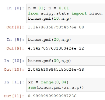
Example 1.3.2: Assume that the probability of a key failing on an 83-set keyboard (the authors, laptop keyboard has 83 keys) is 0.01. Now, we need to find the probability when at a given time there are 10, 20, and 30 non-functioning keys on this keyboard. Using the dbinom function, these probabilities are easy to calculate. Try to do this same problem using a scientific calculator or by writing a simple function in any language that you are comfortable with:
> n <- 83; p <- 0.01
> dbinom(10,n,p)
[1] 1.168e-08
> dbinom(20,n,p)
[1] 4.343e-22
> dbinom(30,n,p)
[1] 2.043e-38
> sum(dbinom(0:83,n,p))
[1] 1
As the probabilities of 10-30 keys failing appear too small, it is natural to believe that maybe something is going wrong. As a check, the sum clearly equals 1. Let us have a look at the problem from a different angle. For many x values, the probability p(x) will be approximately zero. We may not be interested in the probability of an exact number of failures though we are interested in the probability of at least x failures occurring, that is, we are interested in the cumulative probabilities  . The cumulative probabilities for binomial distribution are obtained in R using the
 pbinom function. The main arguments of pbinom include size (for n), prob (for p), and q (the at least x argument). For the same problem, we now look at the cumulative probabilities for various p values:
> n <- 83; p <- seq(0.05,0.95,0.05)
> x <- seq(0,83,5)
> i <- 1
> plot(x,pbinom(x,n,p[i]),”l”,col=1,xlab=”x”,ylab=
+ expression(P(X<=x)))
> for(i in 2:length(p)) { points(x,pbinom(x,n,p[i]),”l”,col=i)}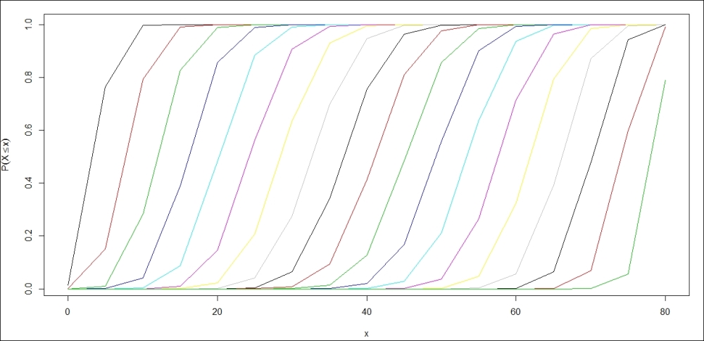
Cumulative binomial probabilities
Try to interpret the preceding figure, the parallel Python program would be the following:
A box of N = 200 pieces of 12 GB pen drives arrives at a sales center. The carton contains M = 20 defective pen drives. A random sample of n units is drawn from the carton. Let X denote the number of defective pen drives obtained from the sample of n units. The task is to obtain the probability distribution of X. The number of possible ways of obtaining the sample of size n is  . In this problem, we have M defective units and N-M working pen drives, and x defective units can be sampled in
  different ways and n-x good units can be obtained in
  distinct ways. Thus, the probability distribution of the RV X is calculated as:
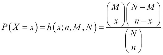
where x is an integer between  and
and  . The RV is called the hypergeometric RV and its probability distribution is called the hypergeometric distribution.
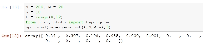
Suppose that we draw a sample of n = 10 units. The dhyper function in R can be used to find the probabilities of the RV X, assuming different values:
> N = 200; M = 20
> n = 10
> x = 0:11
> round(dhyper(x,M,N,n),3)
 [1] 0.377 0.395 0.176 0.044 0.007 0.001 0.000 0.000 0.000 0.000 0.000 0.000
The equivalent Python implementation is as follows:
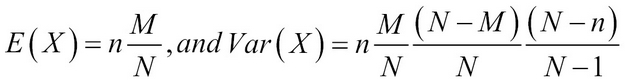
The mean and variance of a hypergeometric distribution are stated as follows:
Consider a variant of the problem described in the previous subsection. The 10 new desktops need to be fitted with an add-on, five megapixel external cameras, to help the students attend a certain online course. Assume that the probability of a non-defective camera unit is p. As an administrator, you keep on placing orders until you receive 10 non-defective cameras. Now, let X denote the number of orders placed for obtaining the 10 good units. We denote the required number of successes by k, which in this discussion has been k = 10. The goal in this unit is to obtain the probability distribution of X.
Suppose that the xth order placed results in the procurement of a kth non-defective unit. This implies that we have received (k-1) non-defective units among the first (x-1) orders placed, which is possible in  distinct ways. At the xth order, the instant of having received the kth non-defective unit, we have k successes and x-k failures. Thus, the probability distribution of the RV is calculated as:
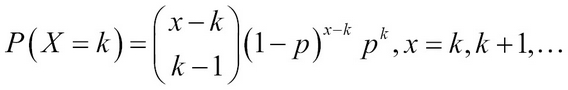
Such an RV is called a negative binomial RV and its probability distribution as the negative binomial distribution. Technically, this RV has no upper bound as the next required success may never turn up. We state the mean and variance of this distribution as follows:
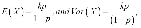
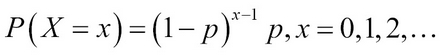
A particular and important special case of the negative binomial RV occurs for k = 1, which is known as the geometric RV. In this case, the pmf is calculated as:
Example 1.3.3. (Baron (2007). Page 77) sequential testing: In a certain setup, the probability of an item being defective is (1-p) = 0.05. To complete the lab setup, 12 non-defective units are required. We need to compute the probability that at least 15 units need to be tested. Here we make use of the cumulative distribution of the negative binomial distribution pnbinom function available in R. Similar to the pbinom function, the main arguments that we require here would be size, prob, and q. This problem is solved in a single line of code:
> 1-pnbinom(3,size=12,0.95)
[1] 0.005467259
Note that we have specified 3 as the quantile point (at least x argument) as the size parameter of this experiment is 12 and we are seeking at least 15 units that translate into three more units than the size of the parameter. The pnbinom function computes the cumulative distribution function and the requirement is actually the complement and hence the expression in the code is 1–pnbinom. We may equivalently solve the problem using the dnbinom function, which straightforwardly computes the required probability:
> 1-(dnbinom(3,size=12,0.95)+dnbinom(2,size=12,0.95)+dnbinom(1,
+ size=12,0.95)+dnbinom(0,size=12,0.95))
[1] 0.005467259
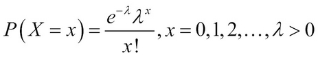
The number of accidents on a 1 km stretch of road, the total calls received during a 1-hour slot on your mobile, the number of "likes” received on a status on a social networking site in a day, and similar other cases, are some of the examples that are addressed by the Poisson RV. The probability distribution of a Poisson RV is calculated as:
Here,  is the parameter of the Poisson RV with X denoting the number of events. The Poisson distribution is sometimes also referred to as the law of rare events. The mean and variance of the Poisson RV are surprisingly the same and equal , that is,
 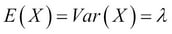 .
.
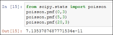
Example 1.3.4: Suppose that Santa commits errors in a software program with a mean of three errors per A4-size page. Santa’s manager wants to know the probability of Santa committing 0, 5, and 20 errors per page. The R function, dpois, helps to determine the answer:
> dpois(0,lambda=3); dpois(5,lambda=3); dpois(20, lambda=3)
[1] 0.04978707
[1] 0.1008188
[1] 7.135379e-11
Note that Santa’s probability of committing 20 errors is almost 0.The Python program is the following:
We will next focus on continuous distributions.