

The first of the three networks we will be looking at is known as a multilayer perceptrons or (MLPs). Let's suppose that the objective is to create a neural network for identifying numbers based on handwritten digits. For example, when the input to the network is an image of a handwritten number 8, the corresponding prediction must also be the digit 8. This is a classic job of classifier networks that can be trained using logistic regression. To both train and validate a classifier network, there must be a sufficiently large dataset of handwritten digits. The Modified National Institute of Standards and Technology dataset or MNIST for short, is often considered as the Hello World! of deep learning and is a suitable dataset for handwritten digit classification.
Before we discuss the multilayer perceptron model, it's essential that we understand the MNIST dataset. A large number of the examples in this book use the MNIST dataset. MNIST is used to explain and validate deep learning theories because the 70,000 samples it contains are small, yet sufficiently rich in information:
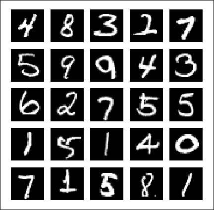
Figure 1.3.1: Example images from the MNIST dataset. Each image is 28 × 28-pixel grayscale.
MNIST is a collection of handwritten digits ranging from the number 0 to 9. It has a training set of 60,000 images, and 10,000 test images that are classified into corresponding categories or labels. In some literature, the term target or ground truth is also used to refer to the label.
In the preceding figure sample images of the MNIST digits, each being sized at 28 X 28-pixel grayscale, can be seen. To use the MNIST dataset in Keras, an API is provided to download and extract images and labels automatically. Listing 1.3.1 demonstrates how to load the MNIST dataset in just one line, allowing us to both count the train and test labels and then plot random digit images.
Listing 1.3.1, mnist-sampler-1.3.1.py. Keras code showing how to access MNIST dataset, plot 25 random samples, and count the number of labels for train and test datasets:
import numpy as np
from keras.datasets import mnist
import matplotlib.pyplot as plt

# load dataset
(x_train, y_train), (x_test, y_test) = mnist.load_data()

# count the number of unique train labels
unique, counts = np.unique(y_train, return_counts=True)
print("Train labels: ", dict(zip(unique, counts)))

# count the number of unique test labels
unique, counts = np.unique(y_test, return_counts=True)
print("Test labels: ", dict(zip(unique, counts)))

# sample 25 mnist digits from train dataset
indexes = np.random.randint(0, x_train.shape[0], size=25)
images = x_train[indexes]
labels = y_train[indexes]

# plot the 25 mnist digits
plt.figure(figsize=(5,5))
for i in range(len(indexes)):
    plt.subplot(5, 5, i + 1)
    image = images[i]
    plt.imshow(image, cmap='gray')
    plt.axis('off')

plt.show()
plt.savefig("mnist-samples.png")
plt.close('all')
The mnist.load_data() method is convenient since there is no need to load all 70,000 images and labels individually and store them in arrays. Executing python3 mnist-sampler-1.3.1.py on command line prints the distribution of labels in the train and test datasets:
Train labels:  {0: 5923, 1: 6742, 2: 5958, 3: 6131, 4: 5842, 5: 5421, 6: 5918, 7: 6265, 8: 5851, 9: 5949}
Test labels:  {0: 980, 1: 1135, 2: 1032, 3: 1010, 4: 982, 5: 892, 6: 958, 7: 1028, 8: 974, 9: 1009}
Afterward, the code will plot 25 random digits as shown in the preceding figure, Figure 1.3.1.
Before discussing the multilayer perceptron classifier model, it is essential to keep in mind that while MNIST data are 2D tensors, they should be reshaped accordingly depending on the type of input layer. The following figure shows how a 3 × 3 grayscale image is reshaped for MLPs, CNNs, and RNNs input layers:
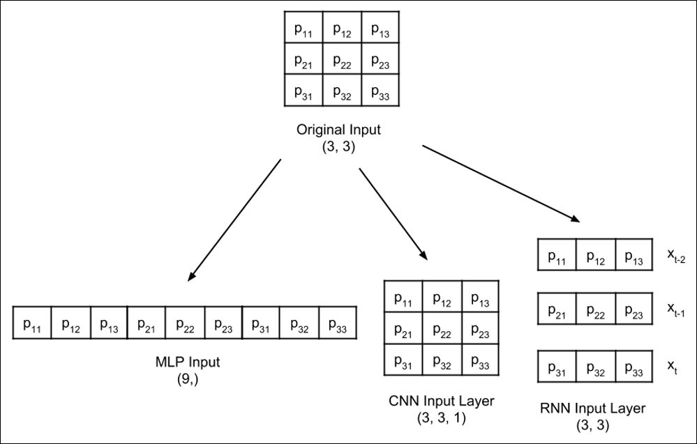
Figure 1.3.2: An input image similar to the MNIST data is reshaped depending on the type of input layer. For simplicity, reshaping of a 3 × 3 grayscale image is shown.
The proposed MLP model shown in Figure 1.3.3 can be used for MNIST digit classification. When the units or perceptrons are exposed, the MLP model is a fully connected network as shown in Figure 1.3.4. It will also be shown how the output of the perceptron is computed from inputs as a function of weights, wi and bias, b n for the nth unit. The corresponding Keras implementation is illustrated in Listing 1.3.2.
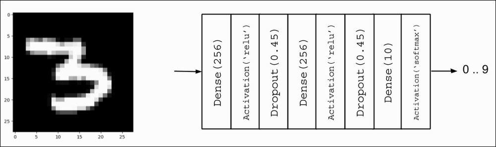
Figure 1.3.3: MLP MNIST digit classifier model
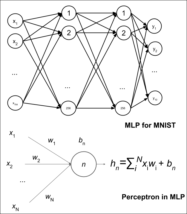
Figure 1.3.4: The MLP MNIST digit classifier in Figure 1.3.3 is made up of fully connected layers. For simplicity, the activation and dropout are not shown. One unit or perceptron is also shown.
Listing 1.3.2, mlp-mnist-1.3.2.py shows the Keras implementation of the MNIST digit classifier model using MLP:
import numpy as np
from keras.models import Sequential
from keras.layers import Dense, Activation, Dropout
from keras.utils import to_categorical, plot_model
from keras.datasets import mnist

# load mnist dataset
(x_train, y_train), (x_test, y_test) = mnist.load_data()

# compute the number of labels
num_labels = len(np.unique(y_train))

# convert to one-hot vector
y_train = to_categorical(y_train)
y_test = to_categorical(y_test)

# image dimensions (assumed square)
image_size = x_train.shape[1]
input_size = image_size * image_size

# resize and normalize
x_train = np.reshape(x_train, [-1, input_size])
x_train = x_train.astype('float32') / 255
x_test = np.reshape(x_test, [-1, input_size])
x_test = x_test.astype('float32') / 255

# network parameters
batch_size = 128
hidden_units = 256
dropout = 0.45

# model is a 3-layer MLP with ReLU and dropout after each layer
model = Sequential()
model.add(Dense(hidden_units, input_dim=input_size))
model.add(Activation('relu'))
model.add(Dropout(dropout))
model.add(Dense(hidden_units))
model.add(Activation('relu'))
model.add(Dropout(dropout))
model.add(Dense(num_labels))
# this is the output for one-hot vector
model.add(Activation('softmax'))
model.summary()
plot_model(model, to_file='mlp-mnist.png', show_shapes=True)

# loss function for one-hot vector
# use of adam optimizer
# accuracy is a good metric for classification tasks
model.compile(loss='categorical_crossentropy',
              optimizer='adam',
              metrics=['accuracy'])
# train the network
model.fit(x_train, y_train, epochs=20, batch_size=batch_size)

# validate the model on test dataset to determine generalization
loss, acc = model.evaluate(x_test, y_test, batch_size=batch_size)
print("\nTest accuracy: %.1f%%" % (100.0 * acc))
Before discussing the model implementation, the data must be in the correct shape and format. After loading the MNIST dataset, the number of labels is computed as:
# compute the number of labels
num_labels = len(np.unique(y_train))
Hard coding num_labels = 10 is also an option. But, it's always a good practice to let the computer do its job. The code assumes that y_train has labels 0 to 9.
At this point, the labels are in digits format, 0 to 9. This sparse scalar representation of labels is not suitable for the neural network prediction layer that outputs probabilities per class. A more suitable format is called a one-hot vector, a 10-dim vector with all elements 0, except for the index of the digit class. For example, if the label is 2, the equivalent one-hot vector is [0,0,1,0,0,0,0,0,0,0]. The first label has index 0.
The following lines convert each label into a one-hot vector:
# convert to one-hot vector
y_train = to_categorical(y_train)
y_test = to_categorical(y_test)
In deep learning, data is stored in tensors. The term tensor applies to a scalar (0D tensor), vector (1D tensor), matrix (2D tensor), and a multi-dimensional tensor. From this point, the term tensor is used unless scalar, vector, or matrix makes the explanation clearer.
The rest computes the image dimensions, input_size of the first Dense layer and scales each pixel value from 0 to 255 to range from 0.0 to 1.0. Although raw pixel values can be used directly, it is better to normalize the input data as to avoid large gradient values that could make training difficult. The output of the network is also normalized. After training, there is an option to put everything back to the integer pixel values by multiplying the output tensor by 255.
The proposed model is based on MLP layers. Therefore, the input is expected to be a 1D tensor. As such, x_train and x_test are reshaped to [60000, 28 * 28] and [10000, 28 * 28], respectively.
# image dimensions (assumed square)
image_size = x_train.shape[1]
input_size = image_size * image_size

# resize and normalize
x_train = np.reshape(x_train, [-1, input_size])
x_train = x_train.astype('float32') / 255
x_test = np.reshape(x_test, [-1, input_size])
x_test = x_test.astype('float32') / 255After data preparation, building the model is next. The proposed model is made of three MLP layers. In Keras, an MLP layer is referred to as Dense, which stands for the densely connected layer. Both the first and second MLP layers are identical in nature with 256 units each, followed by relu activation and dropout. 256 units are chosen since 128, 512 and 1,024 units have lower performance metrics. At 128 units, the network converges quickly, but has a lower test accuracy. The added number units for 512 or 1,024 does not increase the test accuracy significantly.
The number of units is a hyperparameter. It controls the capacity of the network. The capacity is a measure of the complexity of the function that the network can approximate. For example, for polynomials, the degree is the hyperparameter. As the degree increases, the capacity of the function also increases.
As shown in the following model, the classifier model is implemented using a sequential model API of Keras. This is sufficient if the model requires one input and one output processed by a sequence of layers. For simplicity, we'll use this in the meantime, however, in Chapter 2, Deep Neural Networks, the Functional API of Keras will be introduced to implement advanced deep learning models.
# model is a 3-layer MLP with ReLU and dropout after each layer
model = Sequential()
model.add(Dense(hidden_units, input_dim=input_size))
model.add(Activation('relu'))
model.add(Dropout(dropout))
model.add(Dense(hidden_units))
model.add(Activation('relu'))
model.add(Dropout(dropout))
model.add(Dense(num_labels))
# this is the output for one-hot vector
model.add(Activation('softmax'))
Since a Dense layer is a linear operation, a sequence of Dense layers can only approximate a linear function. The problem is that the MNIST digit classification is inherently a non-linear process. Inserting a relu activation between Dense layers will enable MLPs to model non-linear mappings. relu or Rectified Linear Unit (ReLU) is a simple non-linear function. It's very much like a filter that allows positive inputs to pass through unchanged while clamping everything else to zero. Mathematically, relu is expressed in the following equation and plotted in Figure 1.3.5:
relu(x) = max(0,x)
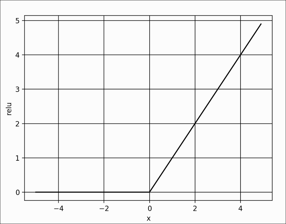
Figure 1.3.5: Plot of ReLU function. The ReLU function introduces non-linearity in neural networks.
There are other non-linear functions that can be used such as elu, selu, softplus, sigmoid, and tanh. However, relu is the most commonly used in the industry and is computationally efficient due to its simplicity. The sigmoid and tanh are used as activation functions in the output layer and described later. Table 1.3.1 shows the equation for each of these activation functions:
|
|
relu(x) = max(0,x) |
1.3.1 |
|
|
softplus(x) = log(1 + e x) |
1.3.2 |
|
|
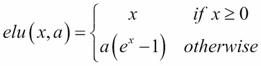 where  and is a tunable hyperparameter |
1.3.3 |
|
|
selu(x) = k × elu(x,a) where k = 1.0507009873554804934193349852946 and a = 1.6732632423543772848170429916717 |
1.3.4 |
Table 1.3.1: Definition of common non-linear activation functions
A neural network has the tendency to memorize its training data especially if it contains more than enough capacity. In such a case, the network fails catastrophically when subjected to the test data. This is the classic case of the network failing to generalize. To avoid this tendency, the model uses a regularizing layer or function. A common regularizing layer is referred to as a dropout.
The idea of dropout is simple. Given a dropout rate (here, it is set to dropout=0.45), the Dropout layer randomly removes that fraction of units from participating in the next layer. For example, if the first layer has 256 units, after dropout=0.45 is applied, only (1 - 0.45) * 256 units = 140 units from layer 1 participate in layer 2. The Dropout layer makes neural networks robust to unforeseen input data because the network is trained to predict correctly, even if some units are missing. It's worth noting that dropout is not used in the output layer and it is only active during training. Moreover, dropout is not present during prediction.
There are regularizers that can be used other than dropouts like l1 or l2. In Keras, the bias, weight and activation output can be regularized per layer. l1 and l2 favor smaller parameter values by adding a penalty function. Both l1 and l2 enforce the penalty using a fraction of the sum of absolute (l1) or square (l2) of parameter values. In other words, the penalty function forces the optimizer to find parameter values that are small. Neural networks with small parameter values are more insensitive to the presence of noise from within the input data.
As an example, l2 weight regularizer with fraction=0.001 can be implemented as:
from keras.regularizers import l2
model.add(Dense(hidden_units,
          kernel_regularizer=l2(0.001),
          input_dim=input_size))
No additional layer is added if l1 or l2 regularization is used. The regularization is imposed in the Dense layer internally. For the proposed model, dropout still has a better performance than l2.
The output layer has 10 units followed by softmax activation. The 10 units correspond to the 10 possible labels, classes or categories. The softmax activation can be expressed mathematically as shown in the following equation:
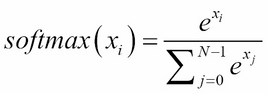
(Equation 1.3.5)
The equation is applied to all N = 10 outputs, x
i
for i = 0, 1 … 9 for the final prediction. The idea of softmax is surprisingly simple. It squashes the outputs into probabilities by normalizing the prediction. Here, each predicted output is a probability that the index is the correct label of the given input image. The sum of all the probabilities for all outputs is 1.0. For example, when the softmax layer generates a prediction, it will be a 10-dim 1D tensor that may look like the following output:
[  3.57351579e-11   7.08998016e-08   2.30154569e-07   6.35787558e-07
   5.57471187e-11   4.15353840e-09   3.55973775e-16   9.99995947e-01
   1.29531730e-09   3.06023480e-06]
The prediction output tensor suggests that the input image is going to be 7 given that its index has the highest probability. The numpy.argmax() method can be used to determine the index of the element with the highest value.
There are other choices of output activation layer, like linear, sigmoid, and tanh. The linear activation is an identity function. It copies its input to its output. The sigmoid function is more specifically known as a logistic sigmoid. This will be used if the elements of the prediction tensor should be mapped between 0.0 and 1.0 independently. The summation of all elements of the predicted tensor is not constrained to 1.0 unlike in softmax. For example, sigmoid is used as the last layer in sentiment prediction (0.0 is bad to 1.0, which is good) or in image generation (0.0 is 0 to 1.0 is 255-pixel values).
The tanh function maps its input in the range -1.0 to 1.0. This is important if the output can swing in both positive and negative values. The tanh function is more popularly used in the internal layer of recurrent neural networks but has also been used as output layer activation. If tanh is used to replace sigmoid in the output activation, the data used must be scaled appropriately. For example, instead of scaling each grayscale pixel in the range [0.0 1.0] using

, it is assigned in the range [-1.0 1.0] by
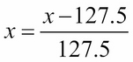
.
The following graph shows the sigmoid and tanh functions. Mathematically, sigmoid can be expressed in equation as follows:
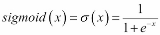
(Equation 1.3.6)
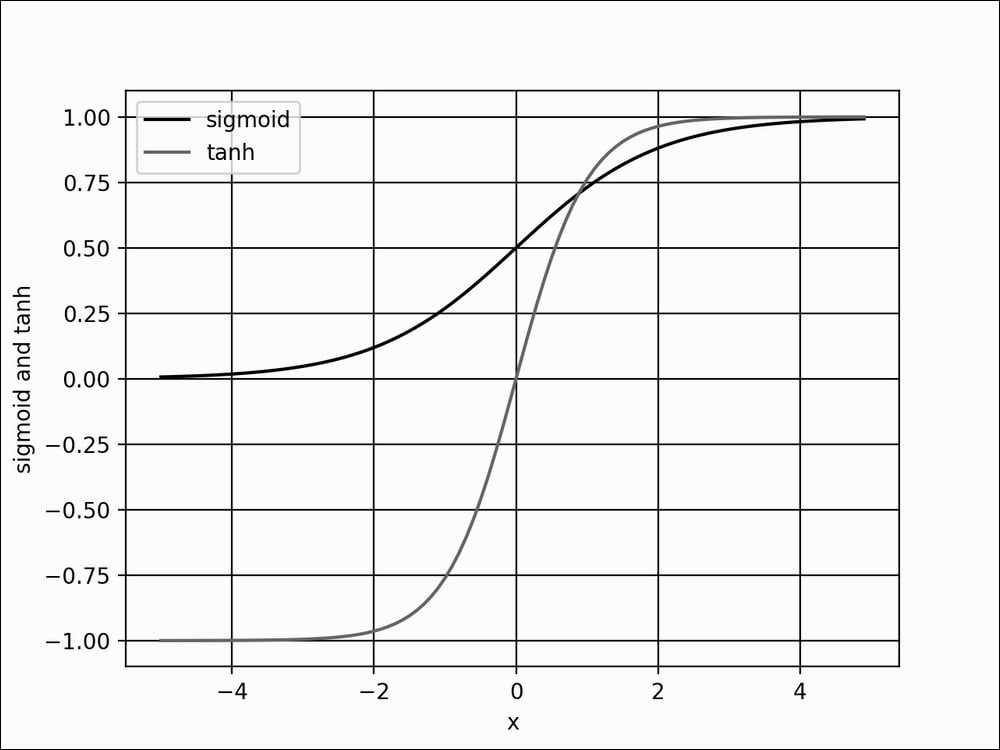
Figure 1.3.6: Plots of sigmoid and tanh
How far the predicted tensor is from the one-hot ground truth vector is called loss. One type of loss function is mean_squared_error (mse), or the average of the squares of the differences between target and prediction. In the current example, we are using categorical_crossentropy. It's the negative of the sum of the product of the target and the logarithm of the prediction. There are other loss functions that are available in Keras, such as mean_absolute_error, and binary_crossentropy. The choice of the loss function is not arbitrary but should be a criterion that the model is learning. For classification by category, categorical_crossentropy or mean_squared_error is a good choice after the softmax activation layer. The binary_crossentropy loss function is normally used after the sigmoid activation layer while mean_squared_error is an option for tanh output.
With optimization, the objective is to minimize the loss function. The idea is that if the loss is reduced to an acceptable level, the model has indirectly learned the function mapping input to output. Performance metrics are used to determine if a model has learned the underlying data distribution. The default metric in Keras is loss. During training, validation, and testing, other metrics such as accuracy can also be included. Accuracy is the percent, or fraction, of correct predictions based on ground truth. In deep learning, there are many other performance metrics. However, it depends on the target application of the model. In literature, performance metrics of the trained model on the test dataset is reported for comparison to other deep learning models.
In Keras, there are several choices for optimizers. The most commonly used optimizers are; Stochastic Gradient Descent (SGD), Adaptive Moments (Adam), and Root Mean Squared Propagation (RMSprop). Each optimizer features tunable parameters like learning rate, momentum, and decay. Adam and RMSprop are variations of SGD with adaptive learning rates. In the proposed classifier network, Adam is used since it has the highest test accuracy.
SGD is considered the most fundamental optimizer. It's a simpler version of the gradient descent in calculus. In gradient descent (GD), tracing the curve of a function downhill finds the minimum value, much like walking downhill in a valley or opposite the gradient until the bottom is reached.
The GD algorithm is illustrated in Figure 1.3.7. Let's suppose x is the parameter (for example, weight) being tuned to find the minimum value of y (for example, loss function). Starting at an arbitrary point of x = -0.5 with the gradient being
. The GD algorithm imposes that x is then updated to
. The new value of x is equal to the old value, plus the opposite of the gradient scaled by


refers to the learning rate. If

, then the new value of x = -0.48.
GD is performed iteratively. At each step, y will get closer to its minimum value. At x = 0.5
, the GD has found the absolute minimum value of y = -1.25. The gradient recommends no further change in x.
The choice of learning rate is crucial. A large value of

may not find the minimum value since the search will just swing back and forth around the minimum value. On the other hand, too small value of

may take a significant number of iterations before the minimum is found. In the case of multiple minima, the search might get stuck in a local minimum.
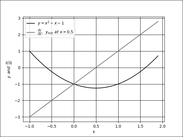
Figure 1.3.7: Gradient descent is similar to walking downhill on the function curve until the lowest point is reached. In this plot, the global minimum is at x = 0.5.
An example of multiple minima can be seen in Figure 1.3.8. If for some reason the search started at the left side of the plot and the learning rate is very small, there is a high probability that GD will find x = -1.51 as the minimum value of y. GD will not find the global minimum at x = 1.66. A sufficiently valued learning rate will enable the gradient descent to overcome the hill at x = 0.0. In deep learning practice, it is normally recommended to start at a bigger learning rate (for example. 0.1 to 0.001) and gradually decrease as the loss gets closer to the minimum.
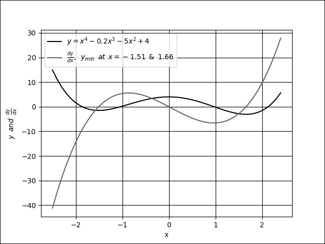
Figure 1.3.8: Plot of a function with 2 minima, x = -1.51 and x = 1.66. Also shown is the derivative of the function.
Gradient descent is not typically used in deep neural networks since you'll often come upon millions of parameters that need to be trained. It is computationally inefficient to perform a full gradient descent. Instead, SGD is used. In SGD, a mini batch of samples is chosen to compute an approximate value of the descent. The parameters (for example, weights and biases) are adjusted by the following equation:
(Equation 1.3.7)
In this equation,

and
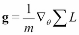
are the parameters and gradients tensor of the loss function respectively. The g is computed from partial derivatives of the loss function. The mini-batch size is recommended to be a power of 2 for GPU optimization purposes. In the proposed network, batch_size=128.
Equation 1.3.7 computes the last layer parameter updates. So, how do we adjust the parameters of the preceding layers? For this case, the chain rule of differentiation is applied to propagate the derivatives to the lower layers and compute the gradients accordingly. This algorithm is known as backpropagation in deep learning. The details of backpropagation are beyond the scope of this book. However, a good online reference can be found at http://neuralnetworksanddeeplearning.com.
Since optimization is based on differentiation, it follows that an important criterion of the loss function is that it must be smooth or differentiable. This is an important constraint to keep in mind when introducing a new loss function.
Given the training dataset, the choice of the loss function, the optimizer, and the regularizer, the model can now be trained by calling the fit() function:
# loss function for one-hot vector
# use of adam optimizer
# accuracy is a good metric for classification tasks
model.compile(loss='categorical_crossentropy',
              optimizer='adam',
              metrics=['accuracy'])
# train the network
model.fit(x_train, y_train, epochs=20, batch_size=batch_size)
This is another helpful feature of Keras. By just supplying both the x and y data, the number of epochs to train, and the batch size, fit() does the rest. In other deep learning frameworks, this translates to multiple tasks such as preparing the input and output data in the proper format, loading, monitoring, and so on. While all of these must be done inside a for loop! In Keras, everything is done in just one line.
In the fit() function, an epoch is the complete sampling of the entire training data. The batch_size parameter is the sample size of the number of inputs to process at each training step. To complete one epoch, fit() requires the size of train dataset divided by batch size, plus 1 to compensate for any fractional part.
At this point, the model for the MNIST digit classifier is now complete. Performance evaluation will be the next crucial step to determine if the proposed model has come up with a satisfactory solution. Training the model for 20 epochs will be sufficient to obtain comparable performance metrics.
The following table, Table 1.3.2, shows the different network configurations and corresponding performance measures. Under Layers, the number of units is shown for layers 1 to 3. For each optimizer, the default parameters in Keras are used. The effects of varying the regularizer, optimizer and number of units per layer can be observed. Another important observation in Table 1.3.2 is that bigger networks do not necessarily translate to better performance.
Increasing the depth of this network shows no added benefits in terms of accuracy for both training and testing datasets. On the other hand, a smaller number of units, like 128, could also lower both the test and train accuracy. The best train accuracy at 99.93% is obtained when the regularizer is removed, and 256 units per layer are used. The test accuracy, however, is much lower at 98.0%, as a result of the network overfitting.
The highest test accuracy is with the Adam optimizer and Dropout(0.45) at 98.5%. Technically, there is still some degree of overfitting given that its training accuracy is 99.39%. Both the train and test accuracy are the same at 98.2% for 256-512-256, Dropout(0.45) and SGD. Removing both the Regularizer and ReLU layers results in it having the worst performance. Generally, we'll find that the Dropout layer has better performance than l2.
Following table demonstrates a typical deep neural network performance during tuning. The example indicates that there is a need to improve the network architecture. In the following section, another model using CNNs shows a significant improvement in test accuracy:
|
Layers |
Regularizer |
Optimizer |
ReLU |
Train Accuracy, % |
Test Accuracy, % |
|---|---|---|---|---|---|
|
256-256-256 |
None |
SGD |
None |
93.65 |
92.5 |
|
256-256-256 |
L2(0.001) |
SGD |
Yes |
99.35 |
98.0 |
|
256-256-256 |
L2(0.01) |
SGD |
Yes |
96.90 |
96.7 |
|
256-256-256 |
None |
SGD |
Yes |
99.93 |
98.0 |
|
256-256-256 |
Dropout(0.4) |
SGD |
Yes |
98.23 |
98.1 |
|
256-256-256 |
Dropout(0.45) |
SGD |
Yes |
98.07 |
98.1 |
|
256-256-256 |
Dropout(0.5) |
SGD |
Yes |
97.68 |
98.1 |
|
256-256-256 |
Dropout(0.6) |
SGD |
Yes |
97.11 |
97.9 |
|
256-512-256 |
Dropout(0.45) |
SGD |
Yes |
98.21 |
98.2 |
|
512-512-512 |
Dropout(0.2) |
SGD |
Yes |
99.45 |
98.3 |
|
512-512-512 |
Dropout(0.4) |
SGD |
Yes |
98.95 |
98.3 |
|
512-1024-512 |
Dropout(0.45) |
SGD |
Yes |
98.90 |
98.2 |
|
1024-1024-1024 |
Dropout(0.4) |
SGD |
Yes |
99.37 |
98.3 |
|
256-256-256 |
Dropout(0.6) |
Adam |
Yes |
98.64 |
98.2 |
|
256-256-256 |
Dropout(0.55) |
Adam |
Yes |
99.02 |
98.3 |
|
256-256-256 |
Dropout(0.45) |
Adam |
Yes |
99.39 |
98.5 |
|
256-256-256 |
Dropout(0.45) |
RMSprop |
Yes |
98.75 |
98.1 |
|
128-128-128 |
Dropout(0.45) |
Adam |
Yes |
98.70 |
97.7 |
Using the Keras library provides us with a quick mechanism to double check the model description by calling:
model.summary()
Listing 1.3.2 shows the model summary of the proposed network. It requires a total of 269,322 parameters. This is substantial considering that we have a simple task of classifying MNIST digits. MLPs are not parameter efficient. The number of parameters can be computed from Figure 1.3.4 by focusing on how the output of the perceptron is computed. From input to Dense layer: 784 × 256 + 256 = 200,960. From first Dense to second Dense: 256 × 256 + 256 = 65,792. From second Dense to the output layer: 10 × 256 + 10 = 2,570. The total is 269,322.
Listing 1.3.2 shows a summary of an MLP MNIST digit classifier model:
_________________________________________________________________
Layer (type)                 Output Shape              Param #
=================================================================
dense_1 (Dense)              (None, 256)               200960
_________________________________________________________________
activation_1 (Activation)    (None, 256)               0
_________________________________________________________________
dropout_1 (Dropout)          (None, 256)               0
_________________________________________________________________
dense_2 (Dense)              (None, 256)               65792
_________________________________________________________________
activation_2 (Activation)    (None, 256)               0
_________________________________________________________________
dropout_2 (Dropout)          (None, 256)               0
_________________________________________________________________
dense_3 (Dense)              (None, 10)                2570
_________________________________________________________________
activation_3 (Activation)    (None, 10)                0
=================================================================
Total params: 269,322
Trainable params: 269,322
Non-trainable params: 0
Another way of verifying the network is by calling:
plot_model(model, to_file='mlp-mnist.png', show_shapes=True)
Figure 1.3.9 shows the plot. You'll find that this is similar to the results of summary() but graphically shows the interconnection and I/O of each layer.
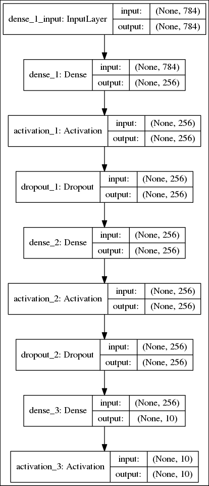
Figure 1.3.9: The graphical description of the MLP MNIST digit classifier