

As we just explained, the simplest neural network is a logistic regressor. A logistic regression takes in values of any range but only outputs values between zero and one.
There is a wide range of applications where logistic regressors are suitable. One such example is to predict the likelihood of a homeowner defaulting on a mortgage.
We might take all kinds of values into account when trying to predict the likelihood of someone defaulting on their payment, such as the debtor's salary, whether they have a car, the security of their job, and so on, but the likelihood will always be a value between zero and one. Even the worst debtor ever cannot have a default likelihood above 100%, and the best cannot go below 0%.
The following diagram shows a logistic regressor. X is our input vector; here it's shown as three components, X1, X2, and X3.
W is a vector of three weights. You can imagine it as the thickness of each of the three lines. W determines how much each of the values of X goes into the next layer. b is the bias, and it can move the output of the layer up or down:
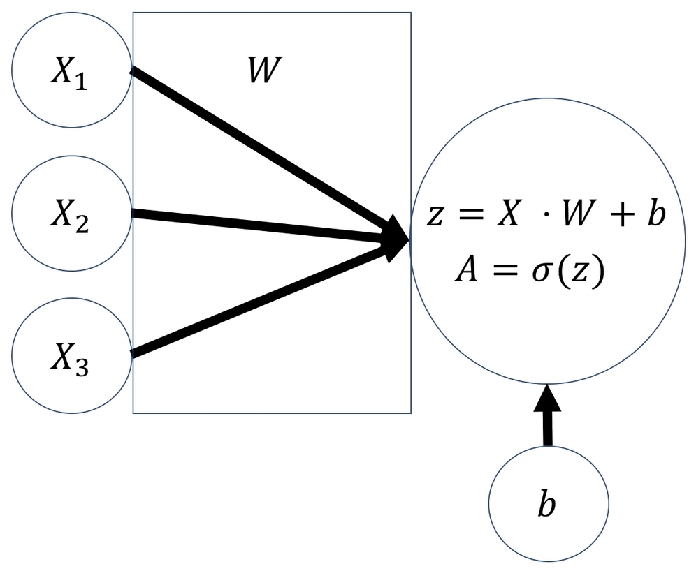
Logistic regressor
To compute the output of the regressor, we must first do a linear step. We compute the dot product of the input, X, and the weights, W. This is the same as multiplying each value of X with its weight and then taking the sum. To this number, we then add the bias, b. Afterward, we do a nonlinear step.
In the nonlinear step, we run the linear intermediate product, z, through an activation function; in this case, the sigmoid function. The sigmoid function squishes the input values to outputs between zero and one:
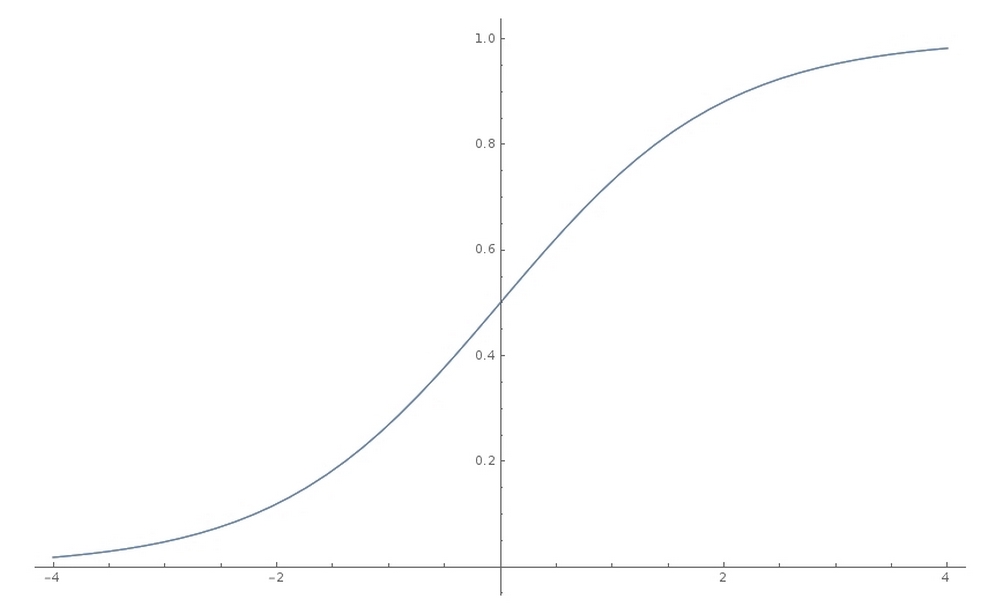
The Sigmoid function
If all the preceding math was a bit too theoretical for you, rejoice! We will now implement the same thing, but this time with Python. In our example, we will be using a library called NumPy, which enables easy and fast matrix operations within Python.
NumPy comes preinstalled with Anaconda and on Kaggle kernels. To ensure we get the same result in all of our experiments, we have to set a random seed. We can do this by running the following code:
import numpy as np
np.random.seed(1)
Since our dataset is quite small, we'll define it manually as NumPy matrices, as we can see here:
X = np.array([[0,1,0],
              [1,0,0],
              [1,1,1],
              [0,1,1]])

y = np.array([[0,1,1,0]]).T
We can define the sigmoid, which squishes all the values into values between 0 and 1, through an activation function as a Python function:
def sigmoid(x):
    return 1/(1+np.exp(-x))
So far, so good. We now need to initialize W. In this case, we actually know already what values W should have. But we cannot know about other problems where we do not know the function yet. So, we need to assign weights randomly.
The weights are usually assigned randomly with a mean of zero, and the bias is usually set to zero by default. NumPy's random function expects to receive the shape of the random matrix to be passed on as a tuple, so random((3,1)) creates a 3x1 matrix. By default, the random values generated are between 0 and 1, with a mean of 0.5 and a standard deviation of 0.5.
We want the random values to have a mean of 0 and a standard deviation of 1, so we first multiply the values generated by 2 and then subtract 1. We can achieve this by running the following code:
W = 2*np.random.random((3,1)) - 1
b = 0
With that done, all the variables are set. We can now move on to do the linear step, which is achieved with the following:
z = X.dot(W) + b
Now we can do the nonlinear step, which is run with the following:
A = sigmoid(z)
Now, if we print out A, we'll get the following output:
print(A)
out:
[[ 0.60841366]
 [ 0.45860596]
 [ 0.3262757 ]
 [ 0.36375058]]
But wait! This output looks nothing like our desired output, y, at all! Clearly, our regressor is representing some function, but it's quite far away from the function we want.
To better approximate our desired function, we have to tweak the weights, W, and the bias, b. To this end, in the next section, we will optimize the model parameters.