Let's see a formal definition of tensors from Wikipedia (https://en.wikipedia.org/wiki/Tensor) as follows:

"Tensors are geometric objects that describe linear relations between geometric vectors, scalars, and other tensors. Elementary examples of such relations include the dot product, the cross product, and linear maps. Geometric vectors, often used in physics and engineering applications, and scalars themselves are also tensors."

This data structure is characterized by three parameters: Rank, Shape, and Type, as shown in the following figure:

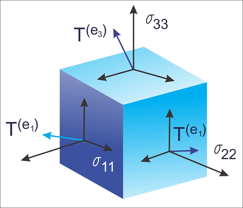
Figure 9: Tensors are nothing but geometrics objects having shape, rank, and type used to hold multidimensional arrays

A tensor thus can be thought of as a generalization of a matrix that specifies an element by an arbitrary number of indices. While practically used, the syntax for tensors is even more or less like nested vectors.

A few people love to compare NumPy versus TensorFlow comparison; however, in reality, TensorFlow and NumPy are quite similar in a sense that both are N-d array libraries!

Well, it's true that NumPy has the n–dimensional array support, but it doesn't offer methods to create tensor functions and automatically compute derivatives (+ no GPU support). The following table can be seen as a short and one-to-one comparison that could make some sense of such comparisons:

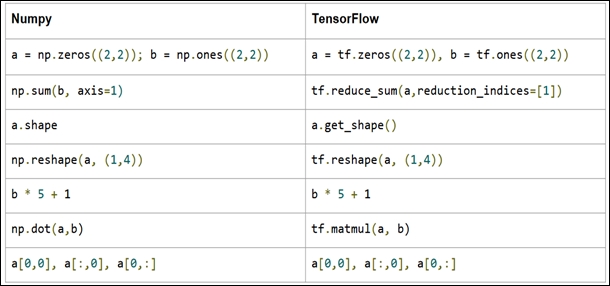
Figure 10: NumPy versus TensorFlow

Now let's see an alternative way of creating tensors before they could be fed (we will see other feeding mechanisms later on) by the TensorFlow graph:

>>> X = [[2.0, 4.0],
        [6.0, 8.0]]
>>> Y = np.array([[2.0, 4.0],
                 [6.0, 6.0]], dtype=np.float32)
>>> Z = tf.constant([[2.0, 4.0],
                    [6.0, 8.0]])

Here X is a list, Y is an n-dimensional array from the NumPy library, and Z is itself the TensorFlow's Tensor object. Now let's see their types:

>>> print(type(X))
>>> print(type(Y))
>>> print(type(Z))
#Output
<class 'list'>
<class 'numpy.ndarray'>
<class 'tensorflow.python.framework.ops.Tensor'>

Well, their types are printed correctly. However, a more convenient function that we're formally dealing with tensors, as opposed to the other types is tf.convert_to_tensor() function as follows:

t1 = tf.convert_to_tensor(X, dtype=tf.float32)t2 = tf.convert_to_tensor(Z, dtype=tf.float32)t3 = tf.convert_to_tensor(Z, dtype=tf.float32)

Now let's see their type using the following lines:

>>> print(type(t1))
>>> print(type(t2))
>>> print(type(t3))
#Output:
<class 'tensorflow.python.framework.ops.Tensor'>
<class 'tensorflow.python.framework.ops.Tensor'>
<class 'tensorflow.python.framework.ops.Tensor'>

Fantastic! I think up to now it's enough discussion already carried out on tensors, so now we can think about the structure that is characterized by the term rank.

Each tensor is described by a unit of dimensionality called rank. It identifies the number of dimensions of the tensor, for this reason, a rank is known as order or n–dimensions of a tensor. A rank zero tensor is a scalar, a rank one tensor id a vector, while a rank two tensor is a matrix. The following code defines a TensorFlow scalar, a vector, a matrix, and a cube_matrix, in the next example we will show how the rank works:

import tensorflow as tf
scalar = tf.constant(100)
vector = tf.constant([1,2,3,4,5])
matrix = tf.constant([[1,2,3],[4,5,6]])
cube_matrix = tf.constant([[[1],[2],[3]],[[4],[5],[6]],[[7],[8],[9]]])
print(scalar.get_shape())
print(vector.get_shape())
print(matrix.get_shape())
print(cube_matrix.get_shape())

The results are printed here:

>>>
()
(5,)
(2, 3)
(3, 3, 1)
>>>

The shape of a tensor is the number of rows and columns it has. Now we will see how to relate the shape to a rank of a tensor:

>>scalar1.get_shape()
TensorShape([])
>>vector1.get_shape()
TensorShape([Dimension(5)])
>>matrix1.get_shape()
TensorShape([Dimension(2), Dimension(3)])
>>cube1.get_shape()
TensorShape([Dimension(3), Dimension(3), Dimension(1)])

In addition to rank and shape, tensors have a data type. The following is the list of the data types:

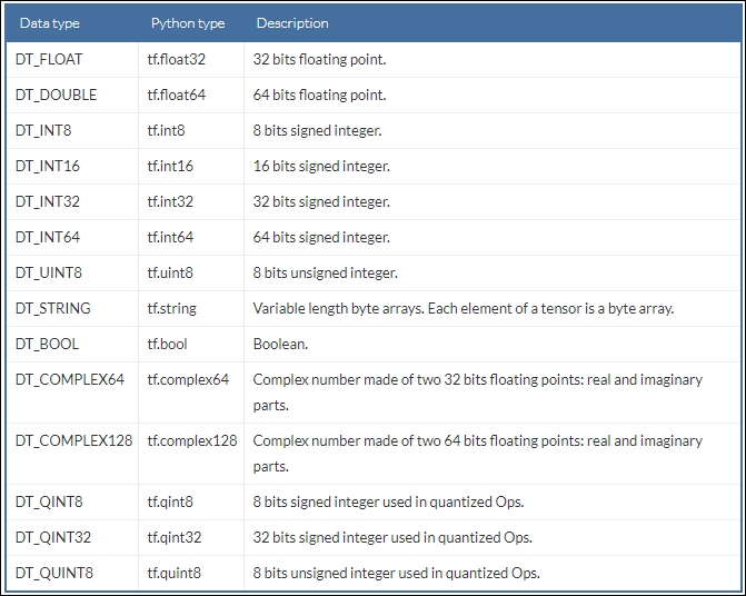
We believe the preceding table is self-explanatory hence we did not provide detailed discussion on the preceding data types. Now the TensorFlow APIs are implemented to manage data to and from NumPy arrays. Thus, to build a tensor with a constant value, pass a NumPy array to the tf.constant() operator, and the result will be a TensorFlow tensor with that value:

import tensorflow as tf
import numpy as np
tensor_1d = np.array([1,2,3,4,5,6,7,8,9,10])
tensor_1d = tf.constant(tensor_1d)
with tf.Session() as sess:
    print (tensor_1d.get_shape())
    print sess.run(tensor_1d)
# Finally, close the TensorFlow session when you're done
sess.close()

Running the example, we obtain:

>>>
 (10,)
 [ 1  2  3  4  5  6  7  8  9 10]

To build a tensor, with variable values, use a NumPy array and pass it to the tf.Variable constructor, the result will be a TensorFlow variable tensor with that initial value:

import tensorflow as tf
import numpy as np
tensor_2d = np.array([(1,2,3),(4,5,6),(7,8,9)])
tensor_2d = tf.Variable(tensor_2d)
with tf.Session() as sess:
    sess.run(tf.global_variables_initializer())
    print (tensor_2d.get_shape())
    print sess.run(tensor_2d)
# Finally, close the TensorFlow session when you're done
sess.close()

The result is:

>>>
 (3, 3)
 [[1 2 3]
 [4 5 6]
 [7 8 9]]

For ease of use in interactive Python environments, we can use the InteractiveSession class, and then use that session for all Tensor.eval() and Operation.run() calls:

import tensorflow as tf
import numpy as np

interactive_session = tf.InteractiveSession()
tensor = np.array([1,2,3,4,5])
tensor = tf.constant(tensor)
print(tensor.eval())

interactive_session.close()

The result is:

>>>
   [1 2 3 4 5]

This can be easier in an interactive setting, such as the shell or an IPython notebook, when it's tedious to pass around a session object everywhere.

Another way to define a tensor is using the TensorFlow statement tf.convert_to_tensor:

import tensorflow as tf
import numpy as np
tensor_3d = np.array([[[0, 1, 2], [3, 4, 5], [6, 7, 8]],
					[[9, 10, 11], [12, 13, 14], [15, 16, 17]],
					[[18, 19, 20], [21, 22, 23], [24, 25, 26]]])
tensor_3d = tf.convert_to_tensor(tensor_3d, dtype=tf.float64)
with tf.Session() as sess:
    print(tensor_3d.get_shape())
    print(sess.run(tensor_3d))
# Finally, close the TensorFlow session when you're done
sess.close()
>>>
(3, 3, 3)
[[[  0.   1.   2.]
  [  3.   4.   5.]
  [  6.   7.   8.]]
 [[  9.  10.  11.]
  [ 12.  13.  14.]
  [ 15.  16.  17.]]
 [[ 18.  19.  20.]
  [ 21.  22.  23.]
  [ 24.  25.  26.]]]

Variables are TensorFlow objects to hold and update parameters. A variable must be initialized; also you can save and restore it to analyze your code. Variables are created by using the tf.Variable() statement. In the following example, we want to count the numbers from 1 to 10, but let's import TensorFlow first:

import tensorflow as tf

We created a variable that will be initialized to the scalar value 0:

value = tf.Variable(0, name="value")

The assign() and add()operators are just nodes of the computation graph, so they do not execute the assignment until the run of the session:

one = tf.constant(1)
new_value = tf.add(value, one)
update_value = tf.assign(value, new_value)
initialize_var = tf.global_variables_initializer()

We can instantiate the computation graph:

with tf.Session() as sess:
    sess.run(initialize_var)
    print(sess.run(value))
    for _ in range(5):
        sess.run(update_value)
        print(sess.run(value))
# Finally, close the TensorFlow session when you're done:
sess.close()

Let's recall that a tensor object is a symbolic handle to the result of an operation, but it does not actually hold the values of the operation's output:

>>>
0
1
2
3
4
5

To fetch the outputs of operations, execute the graph by calling run() on the session object and pass in the tensors to retrieve. Except fetching the single tensor node, you can also fetch multiple tensors. In the following example, the sum and multiply tensors are fetched together, using the run() call:

import tensorflow as tf

constant_A = tf.constant([100.0])
constant_B = tf.constant([300.0])
constant_C = tf.constant([3.0])

sum_ = tf.add(constant_A,constant_B)
mul_ = tf.multiply(constant_A,constant_C)

with tf.Session() as sess:
    result = sess.run([sum_,mul_])
    print(result)

# Finally, close the TensorFlow session when you're done:
sess.close()

The output is as follows:

>>>
[array(400.],dtype=float32),array([ 300.],dtype=float32)]

All the ops needed to produce the values of the requested tensors are run once (not once per requested tensor).

There are four methods of getting data into a TensorFlow program (see details at https://www.tensorflow.org/api_guides/python/reading_data):

In this section, we will see an example of the feeding mechanism only. For the other methods, we will see them in upcoming lesson. TensorFlow provides the feed mechanism that allows us inject data into any tensor in a computation graph. You can provide the feed data through the feed_dict argument to a run() or eval()invoke that initiates the computation.

We can also replace any tensor with feed data (that is variables and constants), the best practice is to use a TensorFlow placeholder node using tf.placeholder() invocation. A placeholder exists exclusively to serve as the target of feeds. An empty placeholder is not initialized so it does not contain any data. Therefore, it will always generate an error if it is executed without a feed, so you won't forget to feed it.

The following example shows how to feed data to build a random 2×3 matrix:

import tensorflow as tf
import numpy as np

a = 3
b = 2
x = tf.placeholder(tf.float32,shape=(a,b))
y = tf.add(x,x)

data = np.random.rand(a,b)
sess = tf.Session()
print sess.run(y,feed_dict={x:data})

# Finally, close the TensorFlow session when you're done:
sess.close()

The output is:

>>>
[[ 1.78602004  1.64606333]
 [ 1.03966308  0.99269408]
 [ 0.98822606  1.50157797]]
>>>