

In this section, we first demonstrate the usefulness of Jupyter Notebooks with examples and through discussion. Then, in order to cover the fundamentals of Jupyter Notebooks for beginners, we'll see the basic usage of them in terms of launching and interacting with the platform. For those who have used Jupyter Notebooks before, this will be mostly a review; however, you will certainly see new things in this topic as well.
Jupyter Notebooks are locally run web applications which contain live code, equations, figures, interactive apps, and Markdown text. The standard language is Python, and that's what we'll be using for this book; however, note that a variety of alternatives are supported. This includes the other dominant data science language, R:
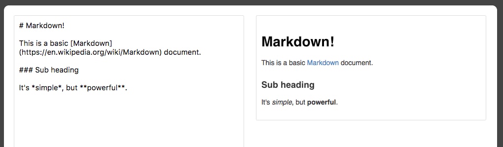
Those familiar with R will know about R Markdown. Markdown documents allow for Markdown-formatted text to be combined with executable code. Markdown is a simple language used for styling text on the web. For example, most GitHub repositories have a README.md Markdown file. This format is useful for basic text formatting. It's comparable to HTML but allows for much less customization. Commonly used symbols in Markdown include hashes (#) to make text into a heading, square and round brackets to insert hyperlinks, and stars to create italicized or bold text:
Having seen the basics of Markdown, let's come back to R Markdown, where Markdown text can be written alongside executable code. Jupyter Notebooks offer the equivalent functionality for Python, although, as we'll see, they function quite differently than R Markdown documents. For example, R Markdown assumes you are writing Markdown unless otherwise specified, whereas Jupyter Notebooks assume you are inputting code. This makes it more appealing to use Jupyter Notebooks for rapid development and testing.
From a data science perspective, there are two primary types for a Jupyter Notebook depending on how they are used: lab-style and deliverable.
Lab-style Notebooks are meant to serve as the programming analog of research journals. These should contain all the work you've done to load, process, analyze, and model the data. The idea here is to document everything you've done for future reference, so it's usually not advisable to delete or alter previous lab-style Notebooks. It's also a good idea to accumulate multiple date-stamped versions of the Notebook as you progress through the analysis, in case you want to look back at previous states.
Deliverable Notebooks are intended to be presentable and should contain only select parts of the lab-style Notebooks. For example, this could be an interesting discovery to share with your colleagues, an in-depth report of your analysis for a manager, or a summary of the key findings for stakeholders.
In either case, an important concept is reproducibility. If you've been diligent in documenting your software versions, anyone receiving the reports will be able to rerun the Notebook and compute the same results as you did. In the scientific community, where reproducibility is becoming increasingly difficult, this is a breath of fresh air.
Now, we are going to open up a Jupyter Notebook and start to learn the interface. Here, we will assume you have no prior knowledge of the platform and go over the basic usage.
Navigate to the companion material directory in the terminal.
Note
On Unix machines such as Mac or Linux, command-line navigation can be done using
lsto display directory contents andcdto change directories.On Windows machines, use
dirto display directory contents and usecdto change directories instead. If, for example, you want to change the drive fromC:toD:, you should executed:to change drives.Start a new local Notebook server here by typing the following into the terminal:
jupyter notebook
A new window or tab of your default browser will open the Notebook Dashboard to the working directory. Here, you will see a list of folders and files contained therein.
Click on a folder to navigate to that particular path and open a file by clicking on it. Although its main use is editing IPYNB Notebook files, Jupyter functions as a standard text editor as well.
Reopen the terminal window used to launch the app. We can see the
NotebookAppbeing run on a local server. In particular, you should see a line like this:[I 20:03:01.045 NotebookApp] The Jupyter Notebook is running at: http://localhost:8888/ ?token=e915bb06866f19ce462d959a9193a94c7c088e81765f9d8a
Going to that HTTP address will load the app in your browser window, as was done automatically when starting the app. Closing the window does not stop the app; this should be done from the terminal by typing Ctrl + C.
Close the app by typing Ctrl + C in the terminal. You may also have to confirm by entering
y. Close the web browser window as well.When loading the NotebookApp, there are various options available to you. In the terminal, see the list of available options by running the following:
jupyter notebook –-help
One such option is to specify a specific port. Open a
NotebookAppat local port9000by running the following:jupyter notebook --port 9000
The primary way to create a new Jupyter Notebook is from the Jupyter Dashboard. Click New in the upper-right corner and select a kernel from the drop-down menu (that is, select something in the Notebooks section):
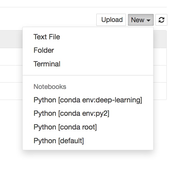
Kernels provide programming language support for the Notebook. If you have installed Python with Anaconda, that version should be the default kernel. Conda virtual environments will also be available here.
Note
Virtual environments are a great tool for managing multiple projects on the same machine. Each virtual environment may contain a different version of Python and external libraries. Python has built-in virtual environments; however, the Conda virtual environment integrates better with Jupyter Notebooks and boasts other nice features. The documentation is available at: https://conda.io/docs/user-guide/tasks/manage-environments.html.
With the newly created blank Notebook, click in the top cell and type
print('hello world'), or any other code snippet that writes to the screen. Execute it by clicking in the cell and pressing Shift + Enter, or by selecting Run Cell in the Cell menu.Any
stdoutorstderroutput from the code will be displayed beneath as the cell runs. Furthermore, the string representation of the object written in the final line will be displayed as well. This is very handy, especially for displaying tables, but sometimes we don't want the final object to be displayed. In such cases, a semicolon (;) can be added to the end of the line to suppress the display.New cells expect and run code input by default; however, they can be changed to render Markdown instead.
Click into an empty cell and change it to accept Markdown-formatted text. This can be done from the drop-down menu icon in the toolbar or by selecting Markdown from the Cell menu. Write some text in here (any text will do), making sure to utilize Markdown formatting symbols such as
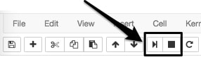
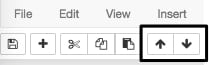
#.Focus on the toolbar at the top of the Notebook:
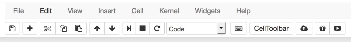
There is a Play icon in the toolbar, which can be used to run cells. As we'll see later, however, it's handier to use the keyboard shortcut Shift + Enter to run cells. Right next to this is a Stop icon, which can be used to stop cells from running. This is useful, for example, if a cell is taking too long to run:
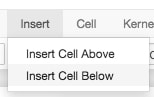
New cells can be manually added from the Insert menu:
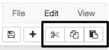
Cells can be copied, pasted, and deleted using icons or by selecting options from the Edit menu:
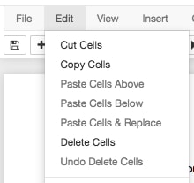
Cells can also be moved up and down this way:
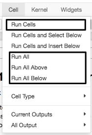
There are useful options under the Cell menu to run a group of cells or the entire Notebook:
Experiment with the toolbar options to move cells up and down, insert new cells, and delete cells.
An important thing to understand about these Notebooks is the shared memory between cells. It's quite simple: every cell existing on the sheet has access to the global set of variables. So, for example, a function defined in one cell could be called from any other, and the same applies to variables. As one would expect, anything within the scope of a function will not be a global variable and can only be accessed from within that specific function.
Open the Kernel menu to see the selections. The Kernel menu is useful for stopping script executions and restarting the Notebook if the kernel dies. Kernels can also be swapped here at any time, but it is unadvisable to use multiple kernels for a single Notebook due to reproducibility concerns.
Open the File menu to see the selections. The File menu contains options for downloading the Notebook in various formats. In particular, it's recommended to save an HTML version of your Notebook, where the content is rendered statically and can be opened and viewed "as you would expect" in web browsers.
The Notebook name will be displayed in the upper-left corner. New Notebooks will automatically be named Untitled.
Change the name of your IPYNB Notebook file by clicking on the current name in the upper-left corner and typing the new name. Then, save the file.
Close the current tab in your web browser (exiting the Notebook) and go to the Jupyter Dashboard tab, which should still be open. (If it's not open, then reload it by copy and pasting the HTTP link from the terminal.)
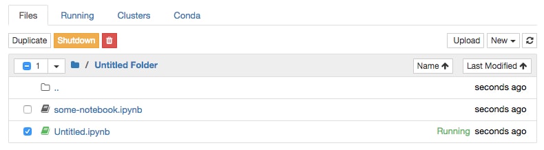
Since we didn't shut down the Notebook, we just saved and exited, it will have a green book symbol next to its name in the Files section of the Jupyter Dashboard and will be listed as Running on the right side next to the last modified date. Notebooks can be shut down from here.
Quit the Notebook you have been working on by selecting it (checkbox to the left of the name) and clicking the orange Shutdown button:
Note
If you plan to spend a lot of time working with Jupyter Notebooks, it's worthwhile to learn the keyboard shortcuts. This will speed up your workflow considerably. Particularly useful commands to learn are the shortcuts for manually adding new cells and converting cells from code to Markdown formatting. Click on Keyboard Shortcuts from the Help menu to see how.
Jupyter has many appealing features that make for efficient Python programming. These include an assortment of things, from methods for viewing docstrings to executing Bash commands. Let's explore some of these features together in this section.
Note
The official IPython documentation can be found here: http://ipython.readthedocs.io/en/stable/. It has details on the features we will discuss here and others.
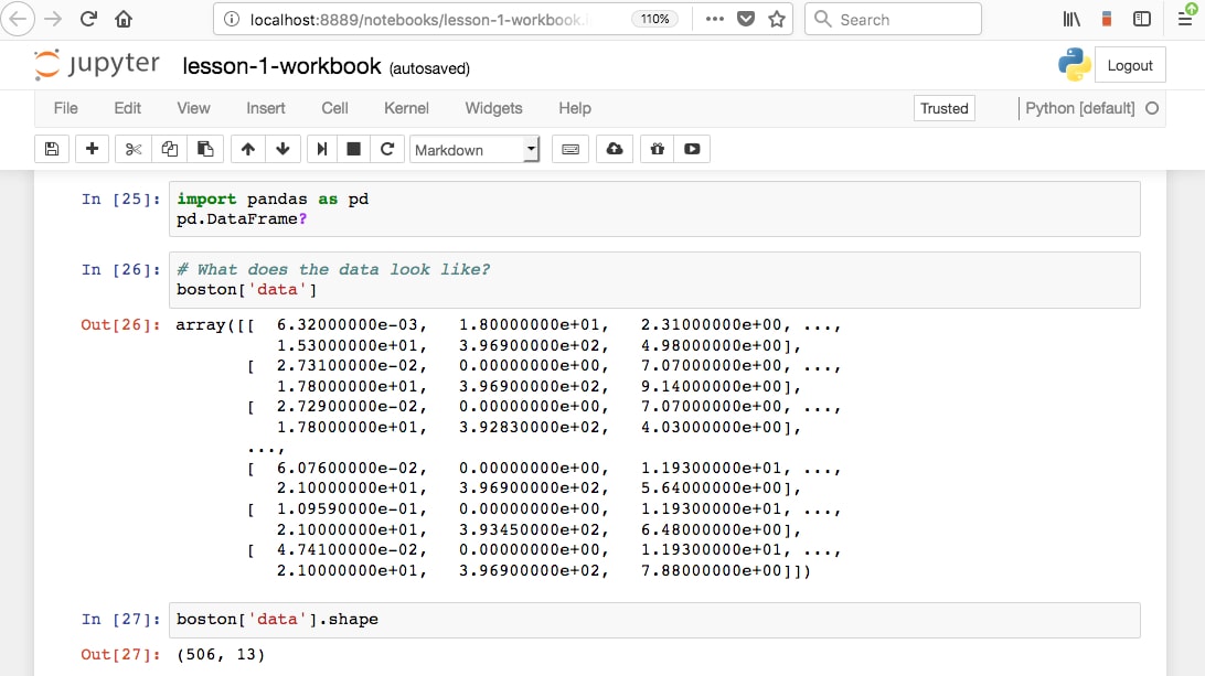
From the Jupyter Dashboard, navigate to the
lesson-1directory and open thelesson-1-workbook.ipynbfile by selecting it. The standard file extension for Jupyter Notebooks is.ipynb, which was introduced back when they were called IPython Notebooks.Scroll down to
Subtopic C: Jupyter Featuresin the Jupyter Notebook. We start by reviewing the basic keyboard shortcuts. These are especially helpful to avoid having to use the mouse so often, which will greatly speed up the workflow. Here are the most useful keyboard shortcuts. Learning to use these will greatly improve your experience with Jupyter Notebooks as well as your own efficiency:Shift + Enter is used to run a cell
The Esc key is used to leave a cell
The M key is used to change a cell to Markdown (after pressing Esc)
The Y key is used to change a cell to code (after pressing Esc)
Arrow keys move cells (after pressing Esc)
The Enter key is used to enter a cell
Moving on from shortcuts, the help option is useful for beginners and experienced coders alike. It can help provide guidance at each uncertain step.
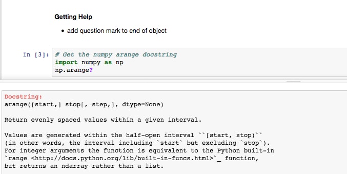
Users can get help by adding a question mark to the end of any object and running the cell. Jupyter finds the docstring for that object and returns it in a pop-out window at the bottom of the app.
Run the Getting Help section cells and check out how Jupyter displays the docstrings at the bottom of the Notebook. Add a cell in this section and get help on the object of your choice:
Tab completion can be used to do the following:
List available modules when importing external libraries
List available modules of imported external libraries
Function and variable completion
This can be especially useful when you need to know the available input arguments for a module, when exploring a new library, to discover new modules, or simply to speed up workflow. They will save time writing out variable names or functions and reduce bugs from typos. The tab completion works so well that you may have difficulty coding Python in other editors after today!
Click into an empty code cell in the Tab Completion section and try using tab completion in the ways suggested immediately above. For example, the first suggestion can be done by typing
import(including the space after) and then pressing the Tab key: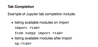
Last but not least of the basic Jupyter Notebook features are magic commands. These consist of one or two percent signs followed by the command. Magics starting with
%%will apply to the entire cell, and magics starting with%will only apply to that line. This will make sense when seen in an example.Scroll to the Jupyter Magic Functions section and run the cells containing
%lsmagicand%matplotlib inline: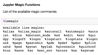
%lsmagiclists the available options. We will discuss and show examples of some of the most useful ones. The most common magic command you will probably see is%matplotlib inline, which allows matplotlib figures to be displayed in the Notebook without having to explicitly useplt.show().The timing functions are very handy and come in two varieties: a standard timer (
%timeor%%time) and a timer that measures the average runtime of many iterations (%timeitand%%timeit).Run the cells in the Timers section. Note the difference between using one and two percent signs.
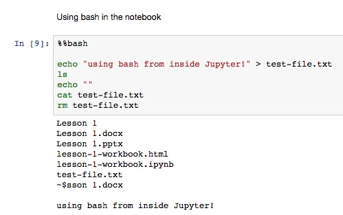
Even by using a Python kernel (as you are currently doing), other languages can be invoked using magic commands. The built-in options include JavaScript, R, Pearl, Ruby, and Bash. Bash is particularly useful, as you can use Unix commands to find out where you are currently (
pwd), what's in the directory (ls), make new folders (mkdir), and write file contents (cat/head/tail).Run the first cell in the Using bash in the notebook section. This cell writes some text to a file in the working directory, prints the directory contents, prints an empty line, and then writes back the contents of the newly created file before removing it:
Run the following cells containing only
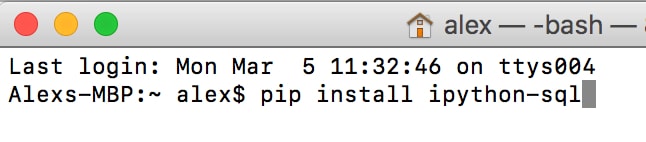
lsandpwd. Note how we did not have to explicitly use the Bash magic command for these to work.There are plenty of external magic commands that can be installed. A popular one is
ipython-sql, which allows for SQL code to be executed in cells.If you've not already done so, install
ipython-sqlnow. Open a new terminal window and execute the following code:pip install ipython-sql
Run the
%load_ext sqlcell to load the external command into the Notebook: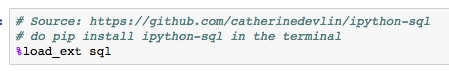
This allows for connections to remote databases so that queries can be executed (and thereby documented) right inside the Notebook.
Run the cell containing the SQL sample query:
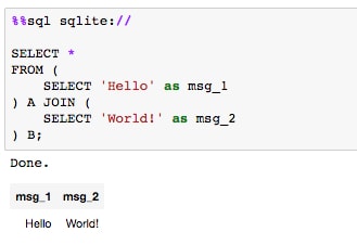
Here, we first connect to the local sqlite source; however, this line could instead point to a specific database on a local or remote server. Then, we execute a simple
SELECTto show how the cell has been converted to run SQL code instead of Python.Moving on to other useful magic functions, we'll briefly discuss one that helps with documentation. The command is
%version_information, but it does not come as standard with Jupyter. Like the SQL one we just saw, it can be installed from the command line withpip.If not already done, install the version documentation tool now from the terminal using
pip. Open up a new window and run the following code:pip install version_information
Once installed, it can then be imported into any Notebook using
%load_ext version_information. Finally, once loaded, it can be used to display the versions of each piece of software in the Notebook.Run the cell that loads and calls the
version_informationcommand: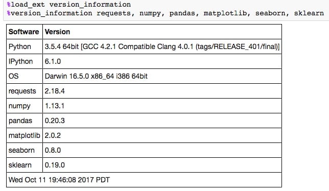
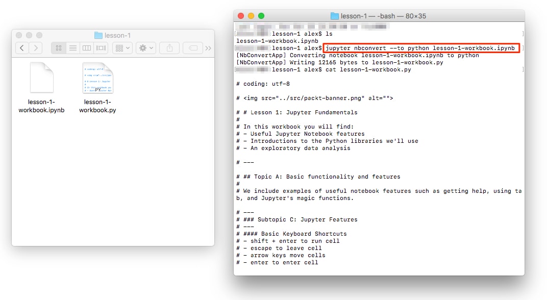
You can convert a Jupyter Notebook to a Python script. This is equivalent to copying and pasting the contents of each code cell into a single .py file. The Markdown sections are also included as comments.
The conversion can be done from the NotebookApp or in the command line as follows:
jupyter nbconvert --to=python lesson-1-notebook.ipynb
This is useful, for example, when you want to determine the library requirements for a Notebook using a tool such as pipreqs. This tool determines the libraries used in a project and exports them into a requirements.txt file (and it can be installed by running pip install pipreqs).
The command is called from outside the folder containing your .py files. For example, if the .py files are inside a folder called lesson-1, you could do the following:
pipreqs lesson-1/
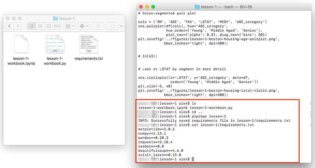
The resulting requirements.txt file for lesson-1-workbook.ipynb looks like this:
cat lesson-1/requirements.txt
matplotlib==2.0.2
numpy==1.13.1
pandas==0.20.3
requests==2.18.4
seaborn==0.8
beautifulsoup4==4.6.0
scikit_learn==0.19.0
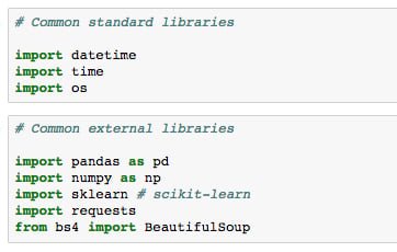
Having now seen all the basics of Jupyter Notebooks, and even some more advanced features, we'll shift our attention to the Python libraries we'll be using in this book. Libraries, in general, extend the default set of Python functions. Examples of commonly used standard libraries are datetime, time, and os. These are called standard libraries because they come standard with every installation of Python.
For data science with Python, the most important libraries are external, which means they do not come standard with Python.
The external data science libraries we'll be using in this book are NumPy, Pandas, Seaborn, matplotlib, scikit-learn, Requests, and Bokeh. Let's briefly introduce each.
Note
It's a good idea to import libraries using industry standards, for example, import numpy as np; this way, your code is more readable. Try to avoid doing things such as from numpy import *, as you may unwittingly overwrite functions. Furthermore, it's often nice to have modules linked to the library via a dot (.) for code readability.
NumPy offers multi-dimensional data structures (arrays) on which operations can be performed far quicker than standard Python data structures (for example, lists). This is done in part by performing operations in the background using C. NumPy also offers various mathematical and data manipulation functions.
Pandas is Python's answer to the R DataFrame. It stores data in 2D tabular structures where columns represent different variables and rows correspond to samples. Pandas provides many handy tools for data wrangling such as filling in NaN entries and computing statistical descriptions of the data. Working with Pandas DataFrames will be a big focus of this book.
Matplotlib is a plotting tool inspired by the MATLAB platform. Those familiar with R can think of it as Python's version of ggplot. It's the most popular Python library for plotting figures and allows for a high level of customization.
Seaborn works as an extension to matplotlib, where various plotting tools useful for data science are included. Generally speaking, this allows for analysis to be done much faster than if you were to create the same things manually with libraries such as matplotlib and scikit-learn.
scikit-learn is the most commonly used machine learning library. It offers top-of-the-line algorithms and a very elegant API where models are instantiated and then fit with data. It also provides data processing modules and other tools useful for predictive analytics.
Requests is the go-to library for making HTTP requests. It makes it straightforward to get HTML from web pages and interface with APIs. For parsing the HTML, many choose BeautifulSoup4, which we will also cover in this book.
Bokeh is an interactive visualization library. It functions similar to matplotlib, but allows us to add hover, zoom, click, and use other interactive tools to our plots. It also allows us to render and play with the plots inside our Jupyter Notebook.
Having introduced these libraries, let's go back to our Notebook and load them, by running the import statements. This will lead us into our first analysis, where we finally start working with a dataset.
Open up the
lesson 1Jupyter Notebook and scroll to theSubtopic D: Python Librariessection.Just like for regular Python scripts, libraries can be imported into the Notebook at any time. It's best practice to put the majority of the packages you use at the top of the file. Sometimes it makes sense to load things midway through the Notebook and that is completely OK.
Run the cells to import the external libraries and set the plotting options:
For a nice Notebook setup, it's often useful to set various options along with the imports at the top. For example, the following can be run to change the figure appearance to something more aesthetically pleasing than the matplotlib and Seaborn defaults:
import matplotlib.pyplot as plt
%matplotlib inline
import seaborn as sns
# See here for more options: https://matplotlib.org/users/customizing.html
%config InlineBackend.figure_format='retina'
sns.set() # Revert to matplotlib defaults
plt.rcParams['figure.figsize'] = (9, 6)
plt.rcParams['axes.labelpad'] = 10
sns.set_style("darkgrid")
So far in this book, we've gone over the basics of using Jupyter Notebooks for data science. We started by exploring the platform and finding our way around the interface. Then, we discussed the most useful features, which include tab completion and magic functions. Finally, we introduced the Python libraries we'll be using in this book.
The next section will be very interactive as we perform our first analysis together using the Jupyter Notebook.