
One of the main reasons Python is a powerful programming language is the libraries and packages that come with it. There are more than 130,000 packages on the Python Package Index (PyPI) and counting! Let's explore some of the libraries and packages that are part of the data science stack.
The components of the data science stack are as follows:
NumPy: A numerical manipulation package
pandas: A data manipulation and analysis library
SciPy library: A collection of mathematical algorithms built on top of NumPy
Matplotlib: A plotting and graph library
IPython: An interactive Python shell
Jupyter notebook: A web document application for interactive computing
The combination of these libraries forms a powerful tool set for handling data manipulation and analysis. We will go through each of the libraries, explore their functionalities, and show how they work together. Let's start with the interpreters.
The IPython shell (https://ipython.org/) is an interactive Python command interpreter that can handle several languages. It allows us to test ideas quickly rather than going through creating files and running them. Most Python installations have a bundled command interpreter, usually called the shell, where you can execute commands iteratively. Although it's handy, this standard Python shell is a bit cumbersome to use. IPython has more features:
Input history that is available between sessions, so when you restart your shell, the previous commands that you typed can be reused.
Using Tab completion for commands and variables, you can type the first letters of a Python command, function, or variable and IPython will autocomplete it.
Magic commands that extend the functionality of the shell. Magic functions can enhance IPython functionality, such as adding a module that can reload imported modules after they are changed in the disk, without having to restart IPython.
Syntax highlighting.
Getting started with the Python shell is simple. Let's follow these steps to interact with the IPython shell:
To start the Python shell, type the ipython command in the console:
> ipython
In [1]:
The IPython shell is now ready and waiting for further commands. First, let's do a simple exercise to solve a sorting problem with one of the basic sorting methods, called straight insertion.
In the IPython shell, copy-paste the following code:
import numpy as np

vec = np.random.randint(0, 100, size=5)
print(vec)
Now, the output for the randomly generated numbers will be similar to the following:
[23, 66, 12, 54, 98, 3]
Use the following logic to print the elements of the vec array in ascending order:
for j in np.arange(1, vec.size):
    v = vec[j]
    i = j
    while i > 0 and vec[i-1] > v:
        vec[i] = vec[i-1]
        i = i - 1
    vec[i] = v
Use the print(vec) command to print the output on the console:
[3, 12, 23, 54, 66, 98]
Now modify the code. Instead of creating an array of 5 elements, change its parameters so it creates an array with 20 elements, using the up arrow to edit the pasted code. After changing the relevant section, use the down arrow to move to the end of the code and press Enter to execute it.
Notice the number on the left, indicating the instruction number. This number always increases. We attributed the value to a variable and executed an operation on that variable, getting the result interactively. We will use IPython in the following sections.
The Jupyter notebook (https://jupyter.org/) started as part of IPython but was separated in version 4 and extended, and lives now as a separate project. The notebook concept is based on the extension of the interactive shell model, creating documents that can run code, show documentation, and present results such as graphs and images.
Jupyter is a web application, so it runs in your web browser directly, without having to install separate software, and enabling it to be used across the internet. Jupyter can use IPython as a kernel for running Python, but it has support for more than 40 kernels that are contributed by the developer community.
Note
A kernel, in Jupyter parlance, is a computation engine that runs the code that is typed into a code cell in a notebook. For example, the IPython kernel executes Python code in a notebook. There are kernels for other languages, such as R and Julia.
It has become a de facto platform for performing operations related to data science from beginners to power users, and from small to large enterprises, and even academia. Its popularity has increased tremendously in the last few years. A Jupyter notebook contains both the input and the output of the code you run on it. It allows text, images, mathematical formulas, and more, and is an excellent platform for developing code and communicating results. Because of its web format, notebooks can be shared over the internet. It also supports the Markdown markup language and renders Markdown text as rich text, with formatting and other features supported.
As we've seen before, each notebook has a kernel. This kernel is the interpreter that will execute the code in the cells. The basic unit of a notebook is called a cell. A cell is a container for either code or text. We have two main types of cells:
Code cell
Markdown cell
A code cell accepts code to be executed in the kernel, displaying the output just below it. A Markdown cell accepts Markdown and will parse the text in Markdown to formatted text when the cell is executed.
Let's run the following exercise to get hands-on experience in the Jupyter notebook.
The fundamental component of a notebook is a cell, which can accept code or text depending on the mode that is selected.
Let's start a notebook to demonstrate how to work with cells, which have two states:
Edit mode
Run mode
When in edit mode, the contents of the cell can be edited, while in run mode, the cell is ready to be executed, either by the kernel or by being parsed to formatted text.
You can add a new cell by using the Insert menu option or using a keyboard shortcut, Ctrl + B. Cells can be converted between Markdown mode and code mode again using the menu or the Y shortcut key for a code cell and M for a Markdown cell.
To execute a cell, click on the Run option or use the Ctrl + Enter shortcut.
Let's execute the following steps to demonstrate how to start to execute simple programs in a Jupyter notebook.
Working with a Jupyter notebook for the first time can be a little confusing, but let's try to explore its interface and functionality. The reference notebook for this exercise is provided on GitHub.
Now, start a Jupyter notebook server and work on it by following these steps:
To start the Jupyter notebook server, run the following command on the console:
> jupyter notebook
After successfully running or installing Jupyter, open a browser window and navigate to http://localhost:8888 to access the notebook.
You should see a notebook similar to the one shown in the following screenshot:
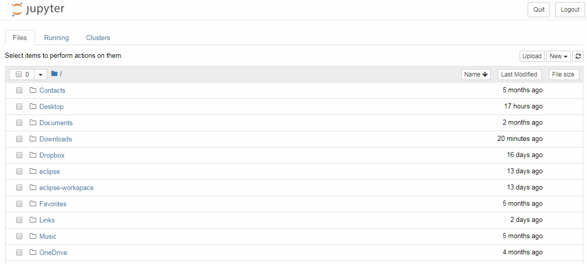
Figure 1.1: Jupyter notebook
After that, from the top-right corner, click on New and select Python 3 from the list.
A new notebook should appear. The first input cell that appears is a Code cell. The default cell type is Code. You can change it via the Cell Type option located under the Cell menu:
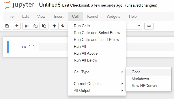
Figure 1.2: Options in the cell menu of Jupyter
Now, in the newly generated Code cell, add the following arithmetic function in the first cell:
In []: x = 2
       print(x*2)
Out []: 4
Now, add a function that returns the arithmetic mean of two numbers, and then execute the cell:
In []: def mean(a,b):
       return (a+b)/2
Let's now use the mean function and call the function with two values, 10 and 20. Execute this cell. What happens? The function is called, and the answer is printed:
In []: mean(10,20)
Out[]: 15.0
We need to document this function. Now, create a new Markdown cell and edit the text in the Markdown cell, documenting what the function does:
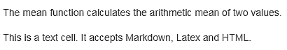
Figure 1.3: Markdown in Jupyter
Then, include an image from the web. The idea is that the notebook is a document that should register all parts of analysis, so sometimes we need to include a diagram or graph from other sources to explain a point.
Now, finally, include the mathematical expression in LaTex in the same Markdown cell:
Figure 1.4: LaTex expression in Jupyter Markdown
As we will see in the rest of the book, the notebook is the cornerstone of our analysis process. The steps that we just followed illustrate the use of different kinds of cells and the different ways we can document our analysis.
Both IPython and Jupyter have a place in the analysis workflow. Usually, the IPython shell is used for quick interaction and more data-heavy work, such as debugging scripts or running asynchronous tasks. Jupyter notebooks, on the other hand, are great for presenting results and generating visual narratives with code, text, and figures. Most of the examples that we will show can be executed in both, except the graphical parts.
IPython is capable of showing graphs, but usually, the inclusion of graphs is more natural in a notebook. We will usually use Jupyter notebooks in this book, but the instructions should also be applicable to IPython notebooks.
Let's demonstrate common Python development in IPython and Jupyter. We will import NumPy, define a function, and iterate the results:
Open the python_script_student.py file in a text editor, copy the contents to a notebook in IPython, and execute the operations.
Copy and paste the code from the Python script into a Jupyter notebook.
Now, update the values of the x and c constants. Then, change the definition of the function.
We now know how to handle functions and change function definitions on the fly in the notebook. This is very helpful when we are exploring and discovering the right approach for some code or an analysis. The iterative approach allowed by the notebook can be very productive in prototyping and faster than writing code to a script and executing that script, checking the results, and changing the script again.
NumPy (http://www.numpy.org) is a package that came from the Python scientific computing community. NumPy is great for manipulating multidimensional arrays and applying linear algebra functions to those arrays. It also has tools to integrate C, C++, and Fortran code, increasing its performance capabilities even more. There are a large number of Python packages that use NumPy as their numerical engine, including pandas and scikit-learn. These packages are part of SciPy, an ecosystem for packages used in mathematics, science, and engineering.
To import the package, open the Jupyter notebook used in the previous activity and type the following command:
import numpy as np
The basic NumPy object is ndarray, a homogeneous multidimensional array, usually composed of numbers, but it can hold generic data. NumPy also includes several functions for array manipulation, linear algebra, matrix operations, statistics, and other areas. One of the ways that NumPy shines is in scientific computing, where matrix and linear algebra operations are common. Another strength of NumPy is its tools that integrate with C++ and FORTRAN code. NumPy is also heavily used by other Python libraries, such as pandas.
SciPy (https://www.scipy.org) is an ecosystem of libraries for mathematics, science, and engineering. NumPy, SciPy, scikit-learn, and others are part of this ecosystem. It is also the name of a library that includes the core functionality for lots of scientific areas.
Matplotlib (https://matplotlib.org) is a plotting library for Python for 2D graphs. It's capable of generating figures in a variety of hard-copy formats for interactive use. It can use native Python data types, NumPy arrays, and pandas DataFrames as data sources. Matplotlib supports several backend—the part that supports the output generation in interactive or file format. This allows Matplotlib to be multiplatform. This flexibility also allows Matplotlib to be extended with toolkits that generate other kinds of plots, such as geographical plots and 3D plots.
The interactive interface for Matplotlib was inspired by the MATLAB plotting interface. It can be accessed via the matplotlib.pyplot module. The file output can write files directly to disk. Matplotlib can be used in scripts, in IPython or Jupyter environments, in web servers, and in other platforms. Matplotlib is sometimes considered low level because several lines of code are needed to generate a plot with more details. One of the tools that we will look at in this book that plots graphs, which are common in analysis, is the Seaborn library, one of the extensions that we mentioned before.
To import the interactive interface, use the following command in the Jupyter notebook:
import matplotlib.pyplot as plt
To have access to the plotting capabilities. We will show how to use Matplotlib in more detail in the next chapter.
Pandas (https://pandas.pydata.org) is a data manipulation and analysis library that's widely used in the data science community. Pandas is designed to work with tabular or labeled data, similar to SQL tables and Excel files.
We will explore the operations that are possible with pandas in more detail. For now, it's important to learn about the two basic pandas data structures: the series, a unidimensional data structure; and the data science workhorse, the bi-dimensional DataFrame, a two-dimensional data structure that supports indexes.
Data in DataFrames and series can be ordered or unordered, homogeneous, or heterogeneous. Other great pandas features are the ability to easily add or remove rows and columns, and operations that SQL users are more familiar with, such as GroupBy, joins, subsetting, and indexing columns. Pandas is also great at handling time series data, with easy and flexible datetime indexing and selection.
Let's import pandas into the Jupyter notebook from the previous activity with the following command:
import pandas as pd