
After creating an intermediate or final dataset in pandas, we can export the values from the DataFrame to several other formats. The most common one is CSV, and the command to do so is df.to_csv('filename.csv'). Other formats, such as Parquet and JSON, are also supported.
Note
Parquet is particularly interesting, and it is one of the big data formats that we will discuss later in the book.
After finishing our analysis, we may want to save our transformed dataset with all the corrections, so if we want to share this dataset or redo our analysis, we don't have to transform the dataset again. We can also include our analysis as part of a larger data pipeline or even use the prepared data in the analysis as input to a machine learning algorithm. We can accomplish data exporting our DataFrame to a file with the right format:
Import all the required libraries and read the data from the dataset using the following command:
import numpy as np
import pandas as pd

url = "https://opendata.socrata.com/api/views/cf4r-dfwe/rows.csv?accessType=DOWNLOAD"
df = pd.read_csv(url)
Redo all adjustments for the data types (date, numeric, and categorical) in the RadNet data. The type should be the same as in Exercise 6: Aggregation and Grouping Data.
Select the numeric columns and the categorical columns, creating a list for each of them:
columns = df.columns
id_cols = ['State', 'Location', "Date Posted", 'Date Collected', 'Sample Type', 'Unit']
columns = list(set(columns) - set(id_cols))
columns
The output is as follows:
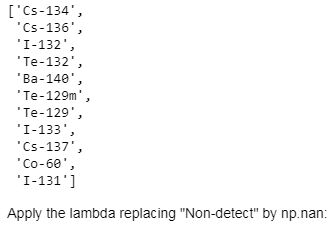
Figure 1.16: List of columns
Apply the lambda function that replaces Non-detect with np.nan:
df['Cs-134'] = df['Cs-134'].apply(lambda x: np.nan if x == "Non-detect" else x)
df.loc[:, columns] = df.loc[:, columns].applymap(lambda x: np.nan if x == 'Non-detect' else x)
df.loc[:, columns] = df.loc[:, columns].applymap(lambda x: np.nan if x == 'ND' else x)
Remove the spaces from the categorical columns:
df.loc[:, ['State', 'Location', 'Sample Type', 'Unit']] = df.loc[:, ['State', 'Location', 'Sample Type', 'Unit']].applymap(lambda x: x.strip())
Transform the date columns to the datetime format:
df['Date Posted'] = pd.to_datetime(df['Date Posted'])
df['Date Collected'] = pd.to_datetime(df['Date Collected'])
Transform all numeric columns to the correct numeric format with the to_numeric method:
for col in columns:
    df[col] = pd.to_numeric(df[col])
Transform all categorical variables to the category type:
df['State'] = df['State'].astype('category')
df['Location'] = df['Location'].astype('category')
df['Unit'] = df['Unit'].astype('category')
df['Sample Type'] = df['Sample Type'].astype('category')
Export our transformed DataFrame, with the right values and columns, to the CSV format with the to_csv function. Exclude the index using index=False, use a semicolon as the separator sep=";", and encode the data as UTF-8 encoding="utf-8":
df.to_csv('radiation_clean.csv', index=False, sep=';', encoding='utf-8')Export the same DataFrame to the Parquet columnar and binary format with the to_parquet method:
df.to_parquet('radiation_clean.prq', index=False)