
In this topic, we will begin fitting our model to the datasets that we have created. In this chapter, we will review the minimum steps required to create a machine learning model that can be applied to building models with any machine learning library, including scikit-learn and Keras.
This book is concerned with applications of deep learning. The vast majority of deep learning tasks are supervised learning, in which there is a given target, and we want to fit a model so that we can understand the relationship between the features and the target.
An example of supervised learning is identifying whether a picture contains a dog or a cat. We want to determine the relationship between the input (a matrix of pixel values) and the target variable, that is, whether the image is of a dog or a cat.
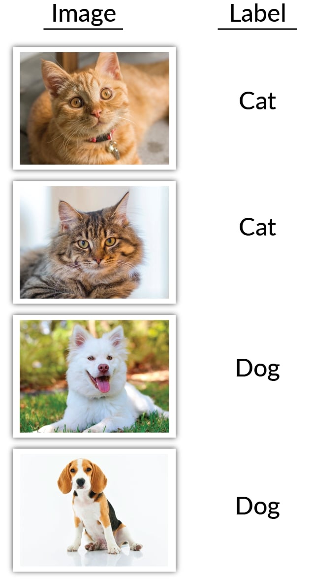
Figure 1.27: A simple supervised learning task to classify images into dogs and cats
Ofcourse, we may need many more images in our training dataset to robustly classify new images, but models that are trained on such a dataset are able to identify the various relationships that differentiate cats and dogs, which can then be used to predict labels for new data.
Supervised learning models are generally used for either classification or regression tasks.
The goal of classification tasks is to fit models from data with discrete categories that can be used to label unlabeled data. For example, these types of models can be used to classify images into dogs or cats. But it doesn't stop at binary classification; multi-label classification is also possible.
Most classification tasks output a probability for each unique class. The prediction is determined as the class with the highest probability, as can be seen in the following figure:
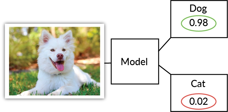
Figure 1.28: An illustration of a classification model labeling an image
Some of the most common classification algorithms are the following:
Logistic regression: This algorithm similar to linear regression, in which feature coefficients are learned and predictions are made by taking the sum of the product of the feature coefficients and features.
Decision trees: This algorithm follows a tree-like structure. Decisions are made at each node and branches represent possible options at the node, terminating in the predicted result.
ANNs: ANNs replicate the structure and performance of a biological neural network to perform pattern recognition tasks. An ANN consists of interconnected neurons, laid out with a set architecture, that pass information to each other until a result is achieved.
While the aim of classification tasks is to label datasets with discrete variables, the aim of regression tasks is to provide input data with continuous variables, and output a numerical value. For example, if you have a dataset of stock market prices, a classification task may predict whether to buy, sell, or hold, whereas a regression task will predict what the stock market price will be.
A simple, yet very popular, algorithm for regression tasks is linear regression. It consists of only one independent feature (x), whose relation with its dependent feature (y) is linear. Due to its simplicity, it is often overlooked, even though it performs very well for simple data problems.
Some of the most common classification algorithms are the following:
Linear regression: This algorithm learns feature coefficients and predictions are made by taking the sum of the product of the feature coefficients and features.
Support Vector Machines: This algorithm uses kernels to map input data into a multi-dimensional feature space to understand relationships between features and the target.
ANNs: ANNs replicate the structure and performance of a biological neural network to perform pattern recognition tasks. An ANN consists of interconnected neurons, laid out with a set architecture, that pass information to each other until a result is achieved.
Whenever we create machine learning models, we separate the data into training and test datasets. The training data is the set of data used to train the model. Typically, it is a large proportion, around 80%, of the total dataset. The test dataset is a sample of the dataset that is held out from the beginning and is used to provide an unbiased evaluation of the model. The test dataset should as accurately as possible represent real-world data. Any model evaluation metrics that are reported should be applied on the test dataset unless it's explicitly stated that the metrics have been evaluated on the training dataset. The reason for this is that models will typically perform better on the data they are trained on. Furthermore, models can overfit the training dataset, meaning that they perform well on the training dataset but perform poorly on the test dataset. A model is said to be overfitted to the data if the model performance is very good when evaluated on the training dataset, but performs poorly on the test dataset. Conversely, a model can be underfitted to the data. In this case, the model will fail to learn relationships between the features and the target, which will lead to poor performance when evaluated on both the training and test datasets. We aim for a balance of the two, not relying so heavily on the training dataset that we overfit, but allowing the model to learn the relationships between features and target so that the model generalizes well to new data. This concept is illustrated in the following figure:
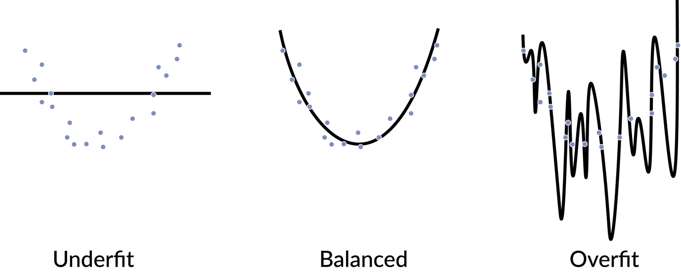
Figure 1.29: A example of under- and overfitting a dataset
There are many ways to split the dataset via sampling methods. One method to split a dataset into training is to simply randomly sample the data until you have the desired number of data points. This is often the default method in functions such as the scikit-learn train_test_spilt function. Another method is to stratify the sampling. In stratified sampling, each subpopulation is sampled independently. Each subpopulation is determined by the target variable. This can be advantageous in examples such as binary classification where the target variable is highly skewed toward one value or another, and random sampling may not provide data points of both values in the training and test datasets. There are also validation datasets, which we will address later in the chapter.
It is important to be able to evaluate our models effectively, not just in terms of the model's performance but also in the context of the problem we are trying to solve. For example, let's say we built a classification task to predict whether to buy, sell, or hold stock based on historical stock market prices. If our model only predicted to buy every time, this would not be a useful result because we may not have infinite resources to buy stocks. It may be better to be less accurate yet also include some sell predictions.
Common evaluation metrics for classification tasks are accuracy, precision, recall, and f1 score. Accuracy is defined as the number of correct predictions divided by the total number of predictions. Accuracy is very interpretable and relatable, and good for when there are balanced classes. When the classes are highly skewed, the accuracy can be misleading, however.
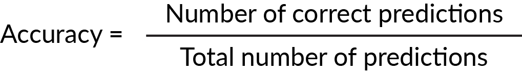
Figure 1.30: Formula to calculate accuracy
Precision is another useful metric. It's defined as the number of true positive results divided by the total number of positive results (true and false) predicted by the model.
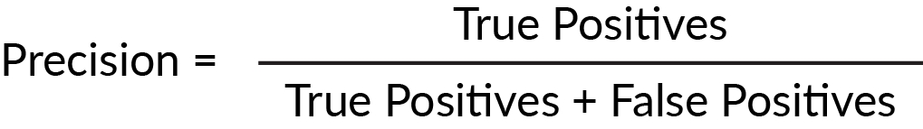
Figure 1.31: Formula to calculate precision
Recall is defined as the number of correct positive results divided by all positive results from the ground truth.

Figure 1.32: Formula to calculate recall
Both precision and recall are scored between zero and one, but scoring well on one may mean scoring poorly on the other. For example, a model may have high precision but low recall, which indicates that the model is very accurate but misses a large number of positive instances. It is useful to have a metric that combines recall and precision. Enter the f1 score, which determines how precise and robust your model is.
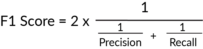
Figure 1.33: Formula to calculate f1 score
When evaluating models, it is helpful to look at a range of different evaluation metrics. They will help determine the most appropriate model and evaluate where the model is misclassifying predictions.
In this exercise, we will create a simple logistic regression model from the scikit-learn package. We will then create some model evaluation metrics and test the predictions against those model evaluation metrics.
We should always approach training any machine learning model training as an iterative approach, beginning first with a simple model, and using model evaluation metrics to evaluate the performance of the models. In this model, our goal is to classify the customers in the bank dataset into training and test datasets:
Load in the data:
import pandas as pd
feats = pd.read_csv('data/bank_data_feats_e3.csv', index_col=0)
target = pd.read_csv('data/bank_data_target_e2.csv', index_col=0)
We first begin by creating a test and train dataset. We will train the data using the training dataset and evaluate the performance of the model on the test dataset.
We will use test_size = 0.2, which means that 20% of the data will be reserved for testing, and we will set a number for the random_state parameter:
from sklearn.model_selection import train_test_split
test_size = 0.2
random_state = 42
X_train, X_test, y_train, y_test = train_test_split(feats, target, test_size=test_size, random_state=random_state)
We can print out the shape of each DataFrame to verify that the dimensions are correct:
print(f'Shape of X_train: {X_train.shape}')
print(f'Shape of y_train: {y_train.shape}')
print(f'Shape of X_test: {X_test.shape}')
print(f'Shape of y_test: {y_test.shape}')
The following figure shows the output of the preceding code:
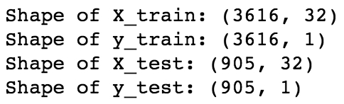
Figure 1.34: Shape of the test and training feature and target DataFrames
These dimensions look correct; each of the target datasets have a single column, the training feature and target DataFrames have the same number of rows, the same applies to the test feature and target DataFrames, and the test DataFrames are 20% of the total dataset.
Next, we have to instantiate our model:
from sklearn.linear_model import LogisticRegression
model = LogisticRegression(random_state=42)
While there are many arguments we can add to scikit-learn's logistic regression model, such as the type and value of regularization parameter, the type of solver, and the maximum number of iterations for the model to have, we will only pass random_state.
We then fit the model to the training data:
model.fit(X_train, y_train['y'])
To test the performance of the model, we compare the predictions of the model with the true values:
y_pred = model.predict(X_test)
There are many types of model evaluation metrics that we can use. Let's start with the accuracy, which is defined as the proportion of predicted values that equal the true values:
from sklearn import metrics
accuracy = metrics.accuracy_score(y_pred=y_pred, y_true=y_test)
print(f'Accuracy of the model is {accuracy*100:.4f}%')
The following figure shows the output of the preceding code:

Figure 1.35: Accuracy of the model
Other common evaluation metrics for classification models are the precision, recall, and f1 score. Scikit-learn has a function that can calculate all three, so we can use that:
precision, recall, fscore, _ = metrics.precision_recall_fscore_support(y_pred=y_pred, y_true=y_test, average='binary')
print(f'Precision: {precision:.4f}\nRecall: {recall:.4f}\nfscore: {fscore:.4f}')
Note
The underscore is used in Python for many reasons. It can be used to recall the value of the last expression in the interpreter, but in this case, we're using it to ignore specific values that are output by the function.
The following figure shows the output of the preceding code:
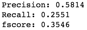
Figure 1.36: The other common evaluation metrics of the model
Since these metrics are scored between 0 and 1, the recall and fscore are not as impressive as the accuracy, though looking at all of these metrics together can help us to find where our models are doing well and where they could be improved by examining in which observations the model gets predictions incorrect.
We can also look at the coefficients that the model outputs to observe which features have a greater impact on the overall result of the prediction:
coef_list = [f'{feature}: {coef}' for coef, feature in sorted(zip(model.coef_[0], X_train.columns.values.tolist()))]
for item in coef_list:
    print(item)
The following figure shows the output of the preceding code:
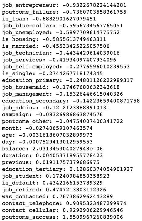
Figure 1.37: The sorted important features of the model with their respective coefficients
This activity has taught us how to create and train a predictive model to predict a target variable given feature variables. We split the feature and target dataset into training and test datasets. Then, we trained our model on the training dataset and evaluated our model on the test dataset. Finally, we observed the trained coefficients for this model.