The goal of this section is introduction of numerous variable types at the first possible occasion. Traditionally, an introductory course begins with the elements of probability theory and then builds up the requisites leading to random variables. This convention is dropped in this book and we begin straightaway with data. There is a primary reason for choosing this path. The approach builds on what the reader is already familiar with and then connects it with the essential framework of the subject.

It is very likely that the user is familiar with questionnaires. A questionnaire may be asked after the birth of a baby with a view to aid the hospital in the study about the experience of the mother, the health status of the baby, and the concerns of immediate guardians of the new born. A multi-store department may instantly request the customer to fill in a short questionnaire for capturing the customer's satisfaction after the sale of a product. A customer's satisfaction following the service of their vehicle (see the detailed example discussed later) can be captured through a few queries. The questionnaires may arise in different forms than just merely on paper. They may be sent via e-mail, telephone, short message service (SMS), and so on. As an example, one may receive an SMS that seeks a mandatory response in a Yes/No form. An e-mail may arrive in the Outlook inbox, which requires the recipient to respond through a vote for any of these three options, "Will attend the meeting", "Can't attend the meeting", or "Not yet decided".

Suppose the owner of a multi-brand car center wants to find out the satisfaction percentage of his customers. Customers bring their car to a service center for varied reasons. The owner wants to find out the satisfaction levels post the servicing of the cars and find the areas where improvement will lead to higher satisfaction among the customers. It is well known that the higher the satisfaction levels, the greater would be the customer's loyalty towards the service center. Towards this, a questionnaire is designed and then data is collected from the customers. A snippet of the questionnaire is given in figure 1, and the information given by the customers lead to different types of data characteristics. The variables Customer ID and Questionnaire ID may be serial numbers or randomly generated unique numbers. The purpose of such variables is unique identification of people's response. It may be possible that there are follow-up questionnaires as well. In such cases, the Customer ID for a responder will continue to be the same, whereas the Questionnaire ID needs to change for identification of the follow up. The values of these types of variables in general are not useful for analytical purpose.

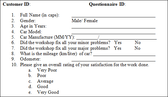
Figure 1: A hypothetical questionnaire

The information of Full Name in this survey is a starting point to break the ice with the responder. In very exceptional cases the name may be useful for profiling purposes. For our purposes the name will simply be a text variable that is not used for analysis purposes. Gender is asked to know the person's gender, and in quite a few cases it may be an important factor explaining the main characteristics of the survey, in this case it may be mileage. Gender is an example of a categorical variable.

Age in Years is a variable that captures the age of the customer. The data for this field is numeric in nature and is an example of a continuous variable.

The fourth and fifth questions help the multi-brand dealer in identifying the car model and its age. The first question here enquires about the type of the car model. The car models of the customers may vary from Volkswagen Beetle, Ford Endeavor, Toyota Corolla, Honda Civic, to Tata Nano, see the next screenshot. Though the model name is actually a noun, we make a distinction from the first question of the questionnaire in the sense that the former is a text variable while the latter leads to a categorical variable. Next, the car model may easily be identified to classify the car into one of the car categories, such as a hatchback, sedan, station wagon, or utility vehicle, and such a classifying variable may serve as one of the ordinal variable, as per the overall car size. The age of the car in months since its manufacture date may explain the mileage and odometer reading.

The sixth and seventh questions simply ask the customer if their minor/major problems were completely fixed or not. This is a binary question that takes either of the values, Yes or No. Small dents, power windows malfunctioning, niggling noises in the cabin, music speakers low output, and other similar issues, which do not lead to good functioning of the car may be treated as minor problems that are expected to be fixed in the car. Disc brake problems, wheel alignment, steering rattling issues, and similar problems that expose the user and co-users of the road to danger are of grave concern, as they affect the functioning of a car and are treated as major problems. Any user will expect all of his/her issues to be resolved during a car service. An important goal of the survey is to find the service center efficiency in handling the minor and major issues of the car. The labels Yes/No may be replaced by +1 and -1, or any other label of convenience.

The eighth question, "What is the mileage (km/liter) of car?", gives a measure of the average petrol/diesel consumption. In many practical cases this data is provided by the belief of the customer who may simply declare it between 5 km/liter to 25 km/liter. In the case of a lower mileage, the customer may ask for a finer tune up of the engine, wheel alignment, and so on. A general belief is that if the mileage is closer to the assured mileage as marketed by the company, or some authority such as Automotive Research Association of India (ARAI), the customer is more likely to be happy. An important variable is the overall kilometers done by the car up to the point of service. Vehicles have certain maintenances at the intervals of 5,000 km, 10,000 km, 20,000 km, 50,000 km, and 100,000 km. This variable may also be related with the age of the vehicle.

Let us now look at the final question of the snippet. Here, the customer is asked to rate his overall experience of the car service. A response from the customer may be sought immediately after a small test ride post the car service, or it may be through a questionnaire sent to the customer's e-mail ID. A rating of Very Poor suggests that the workshop has served the customer miserably, whereas the rating of Very Good conveys that the customer is completely satisfied with the workshop service. Note that there is some order in the response of the customer, in that we can grade the ranking in a certain order of Very Poor < Poor < Average < Good < Very Good. This implies that the structure of the ratings must be respected when we analyze the data of such a study. In the next section, these concepts are elaborated through a hypothetical dataset.

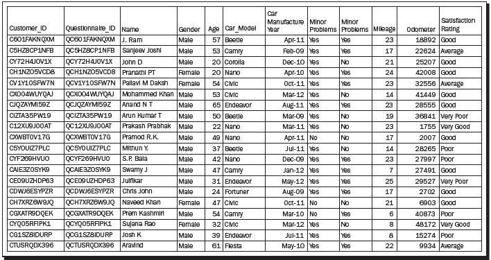
A hypothetical dataset of a Questionnaire

Understanding the data characteristics in an R environment

A snippet of an R session is given in Figure 2. Here we simply relate an R session with the survey and sample data of the previous table. The simple goal here is to get a feel/buy-in of R and not necessarily follow the R codes. The R installation process is explained in the R installation section. Here the user is loading the SQ R data object (SQ simply stands for sample questionnaire) in the session. The nature of the SQ object is a data.frame that stores a variety of other objects in itself. For more technical details of the data.frame function, see The data.frame object section of Chapter 2, Import/Export Data. The names of a data.frame object may be extracted using the function variable.names. The R function class helps to identify the nature of the R object. As we have a list of variables, it is useful to find all of them using the function sapply. In the following screenshot, the mentioned steps have been carried out:

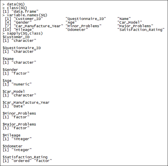
Figure 2: Understanding the variable types of an R object

The variable characteristics are also on expected lines, as they truly should be, and we see that the variables Customer_ID, Questionnaire_ID, and Name are character variables; Gender, Car_Model, Minor_Problems, and Major_Problems are factor variables; DoB and Car_Manufacture_Year are date variables; Mileage and Odometer are integer variables; and finally the variable Satisfaction_Rating is an ordered and factor variable.

In the remainder of this chapter we will delve into more details about the nature of various data types. In a more formal language a variable is called a random variable, abbreviated as RV in the rest of the book, in statistical literature. A distinction needs to be made here. In this book we do not focus on the important aspects of probability theory. It is assumed that the reader is familiar with probability, say at the level of Freund (2003) or Ross (2001). An RV is a function that maps from the probability (sample) space to the real line. From the previous example we have Odometer and Satisfaction_Rating as two examples of a random variable. In a formal language, the random variables are generally denoted by letters X, Y, …. The distinction that is required here is that in the applications what we observe are the realizations/values of the random variables. In general, the realized values are denoted by the lower cases x, y, …. Let us clarify this at more length.

Suppose that we denote the random variable Satisfaction_Rating by X. Here, the sample space consists of the elements Very Poor, Poor, Average, Good, and Very Good. For the sake of convenience we will denote these elements by O₁, O₂, O₃, O₄, and O₅ respectively. The random variable X takes one of the values O₁,…, O₅ with respective probabilities p₁,…, p₅. If the probabilities were known, we don't have to worry about statistical analysis. In simple terms, if we know the probabilities of the Satisfaction_Rating RV, we can simply use it to conclude whether more customers give Very Good rating against Poor. However, our survey data does not contain every customer who have availed car service from the workshop, and as such we have representative probabilities and not actual probabilities. Now, we have seen 20 observations in the R session, and corresponding to each row we had some values under the Satisfaction_Rating column. Let us denote the satisfaction rating for the 20 observations by the symbols X₁,…, X₂₀. Before we collect the data, the random variables X₁,…, X₂₀ can assume any of the values in . Post the data collection, we see that the first customer has given the rating as Good (that is, O₄), the second as Average (O₃), and so on up to the twentieth customer's rating as Average (again O₃). By convention, what is observed in the data sheet is actually X₁,…, x₂₀, the realized values of the RVs X₁,…, X₂₀.