

Attribute relationships define hierarchical dependencies between attributes. A good example is the relationship between attribute City and attribute State. If we know the current city is Phoenix, we know the state must be Arizona. This knowledge of the relationship, City | State, can be used by the Analysis Services engine to optimize performance.
Analysis Services provides the Properties() function to allow us to retrieve data based on attribute relationships.
We will start from a classic Top 10 query that shows the Top 10 Customers. Then we will use the Properties() function to retrieve each top 10 customer's yearly income.
This table shows what our query result should be like:
|
Internet Sales Amount |
Yearly Income | |
|---|---|---|
|
Nichole Nara |
$13,295.38 |
100000 - 120000 |
|
Kaitlyn J. Henderson |
$13,294.27 |
100000 - 120000 |
|
Margaret He |
$13,269.27 |
100000 - 120000 |
|
Randall M. Dominguez |
$13,265.99 |
80000 - 90000 |
|
Adriana L. Gonzalez |
$13,242.70 |
80000 - 90000 |
|
Rosa K. Hu |
$13,215.65 |
40000 - 70000 |
|
Brandi D. Gill |
$13,195.64 |
100000 - 120000 |
|
Brad She |
$13,173.19 |
80000 - 90000 |
|
Francisco A. Sara |
$13,164.64 |
40000 - 70000 |
|
Maurice M. Shan |
$12,909.67 |
80000 - 90000 |
Once we get only the top 10 customers, it's easy enough to place the customer on the rows, and the Internet sales amount on the columns. What about each customer's yearly income?
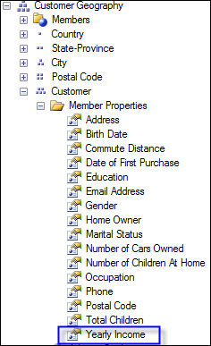
Customer geography is a user-defined hierarchy in the customer dimension. In the SSMS, if you start a new query against the Adventure Works DW 2012 database, and navigate to Customer | Customer Geography | Customer | Member Properties, you will see that the yearly income is one of the member properties for the attribute Customer. This is a good news, because now we can surely get the Yearly Income for each top 10 customer using the PROPERTIES() function:
In SSMS, let us write the following query in a new Query Editor against the Adventure Works DW 2012 database:
This query uses the
TopCount()function which takes three parameters. The first parameter[Customer].[Customer Geography].[Customer].MEMBERSprovides the members that will be evaluated for the "top count", the second integer10tells it to return only 10 members and the third parameter[Measures].[Internet Sales Amount]provides a numeric measure as the evaluation criteria.-- Properties(): Initial SELECT [Measures].[Internet Sales Amount] on 0, TopCount( [Customer].[Customer Geography].[Customer].MEMBERS, 10, [Measures].[Internet Sales Amount] ) ON 1 FROM [Adventure Works]Execute the preceding query, and we should get only 10 customers back with their Internet sales amount. Also notice that the result is sorted in the descending order of the numeric measure. Now let's add a calculated measure, like:
[Customer].[Customer Geography].currentmember.Properties("Yearly Income")To make the calculated measure "dynamic", we must use a member function
.CurrentMember, so we do not need to hardcode any specific member name on the customer dimension. TheProperties()function is also a member function, and it takes another attribute name as a parameter. We've provided "Yearly Income" as the name for the attribute we are interested in.Now place the preceding expression in the
WITHclause, and give it a name[Measures].[Yearly Income]. This new calculated measure is now ready to be placed on the columns axis, along with the Internet sales amount. Here is the final query:WITH MEMBER [Measures].[Yearly Income] AS [Customer].[Customer Geography].currentmember .Properties("Yearly Income") SELECT { [Measures].[Internet Sales Amount], [Measures].[Yearly Income] } on 0, TopCount( [Customer].[Customer Geography].[Customer].MEMBERS, 10, [Measures].[Internet Sales Amount] ) ON 1 FROM [Adventure Works]Executing the query, we should get the yearly income for each top 10 customer. The result should be exactly the same as the table shown at the beginning of our recipe.
Attributes correspond to columns in the dimension tables in our data warehouse. Although we don't normally define the relationship between them, in the relationship database, we do so in the multidimensional space. This knowledge of attribute relationships can be used by the Analysis Services engine to optimize the performance. MDX has provided us the Properties() function to allow us to get from members of one attribute to members of another attribute.
In this recipe, we only focus on one type of member properties, that is, the user-defined member property. Member properties can also be the member properties that are defined by Analysis Services itself, such as NAME, ID, KEY, or CAPTION; they are the intrinsic member properties.
The Properties() function can take another optional parameter, that is the TYPED flag. When the TYPED flag is used, the return value has the original type of the member.
The preceding example does not use the TYPED flag. Without the TYPED flag, the return value is always a string.
In many business analysis, we perform arithmetical operations numerically. In the next example, we will include the TYPED flag in the Properties() function to make sure that the [Total Children] for the top 10 customers are numeric.
WITH
MEMBER [Measures].[Yearly Income] AS
    [Customer].[Customer Geography].currentmember.Properties("Yearly Income")
MEMBER [Measures].[Total Children] AS
    [Customer].[Customer Geography].currentmember.Properties("Total Children", TYPED)
MEMBER [Measures].[Is Numeric] AS
    IIF(
       IsNumeric([Measures].[Total Children]),
       1,
       NULL
       )

SELECT
    { [Measures].[Internet Sales Amount],
      [Measures].[Yearly Income],
      [Measures].[Total Children],
      [Measures].[Is Numeric]
    } ON 0,
    TopCount(
     [Customer].[Customer Geography].[Customer].MEMBERS,
     10,
     [Measures].[Internet Sales Amount]
     ) ON 1
FROM
    [Adventure Works]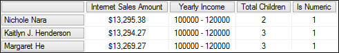
Attributes can be simply referenced as an attribute hierarchy, that is, when the attribute is enabled as an Attribute Hierarchy.
In SSAS, there is one situation where the attribute relationship can be explored only by using the PROPERTIES() function, that is when its property AttributeHierarchyEnabled
is set to False.
In the employee dimension in the Adventure Works cube, employees' SSN numbers are not enabled as an Attribute Hierarchy. Its property AttributeHierarchyEnabled is set to False. We can only reference the SSN number in the PROPERTIES() function of another attribute that has been enabled as Attribute Hierarchy, such as the Employee attribute.