

A common challenge is to find and count reads that have aligned outside of annotated regions. In an RNAseq experiment, these reads can represent non-annotated genes and novel transcripts. Essentially, we have some genes we know about and can see that they are transcribed as they have aligned read coverage, but other transcribed regions do not fall in any annotations and we want to know the locations of the alignments of the reads representing them. In this recipe, we'll look at a deceptively straightforward technique for finding such regions.
Finding unannotated transcribed regions
Getting ready
Our dataset will be a synthetic one that has a small 6,000 bp genome region and two gene features with reads and a third unannotated region with aligning reads, as shown in the following screenshot:
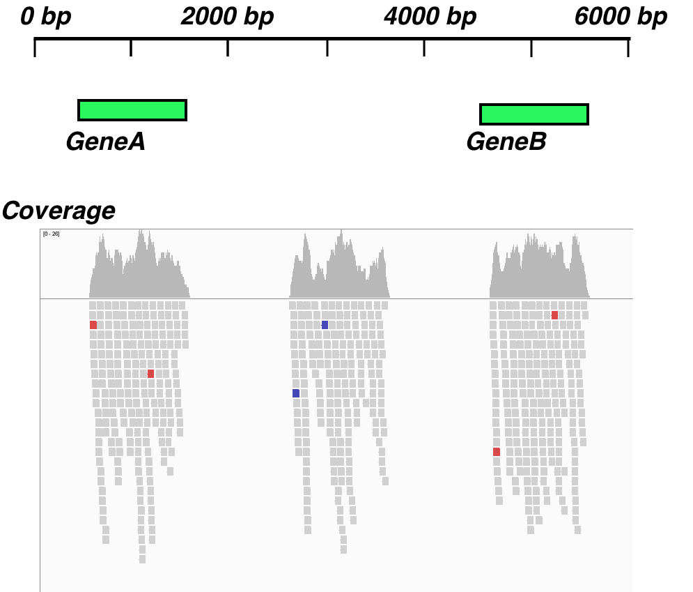
We'll need the Bioconductor csaw, IRanges, SummarizedExperiment, and rtracklayer libraries and some functions from other packages that are part of base Bioconductor. The data is in this book's data repository under datasets/ch1/windows.bam and datasets/ch1/genes.gff
How to do it...
Power analysis with powsimR can be done in the following steps:
- Set up a loading function:
get_annotated_regions_from_gff <- function(file_name) {
    gff <- rtracklayer::import.gff(file_name)
    as(gff, "GRanges")
}
- Get counts in windows across the whole genome:
whole_genome <- csaw::windowCounts(
    file.path(getwd(), "datasets", "ch1", "windows.bam"),
    bin = TRUE,
    filter = 0,
    width = 500,
    param = csaw::readParam(
        minq = 20,
        dedup = TRUE,
        pe = "both"
    )
)
colnames(whole_genome) <- c("small_data")

annotated_regions <- get_annotated_regions_from_gff(file.path(getwd(), "datasets", "ch1", "genes.gff"))
- Find overlaps between annotations and our windows, and subset the windows:
library(IRanges)
library(SummarizedExperiment)
windows_in_genes <-IRanges::overlapsAny( SummarizedExperiment::rowRanges(whole_genome), annotated_regions )
- Subset the windows into those in annotated and non-annotated regions:
annotated_window_counts <- whole_genome[windows_in_genes,]
non_annotated_window_counts <- whole_genome[ ! windows_in_genes,]
- Get the data out to a count matrix:
assay(non_annotated_window_counts)
How it works...
In step 1, we create a function that will load gene region information in a GFF file (see this book's Appendix for a description of GFF) and convert it into a Bioconductor GRanges object using the rtracklayer package. This recipe works because GRanges objects can be subset, just like a regular R matrix or dataframe. They're an object that is "matrix-like" in that respect and although GRanges is much more complicated than a matrix, it behaves much the same. This allows for some easy manipulations and extractions. We use GRanges extensively throughout this recipe, along with the related class, RangedSummarizedExperiment.
In step 2, we use the csaw windowCounts() function to get counts across the whole genome in 500 bp windows. The width parameter defines the window size, and the param parameter determines what constitutes a passing read; here, we set minimum read quality (minq) to a PHRED score of 20, remove PCR duplicates (dedup = TRUE), and require that both of the pairs of a read are aligned (pe="both"). The returned whole_genome object is RangedSummarizedExperiment. We set the name of the single data column in whole_genome to small_data. Finally, we use the custom function, get_annotated_regions_from_gff(), to make a GRanges object, annotated_regions, of the genes represented in our GFF file.
With Step 3, we use the IRanges overlapsAny() function to check whether the window locations overlap at all with the gene regions. This function requires GRanges objects, so we extract that from the whole_genome variable using the SummarizedExperiment rowRanges() function and pass that along with the existing GRanges object's annotated_regions to overlapsAny(). This returns a binary vector that we can use to do subsetting.
In step 4, we simply use the binary vector, windows_in_genes, to subset the whole_genome object, thereby extracting the annotated windows (into annotated_window_counts) as a GRanges object. Then, we can get the non-annotated windows with the same code but by logically inverting the binary vector using the ! operator. This gives us non_annotated_window_counts.
Finally, in step 5, we can extract the actual counts from the GRanges object using the assay() function.
There's more...
We may need to get annotated regions from other file formats than GFF. rtracklayer supports various formats—here's a function for working with BED files:
get_annotated_regions_from_bed <- function(file_name){
    bed <- rtracklayer::import.bed(file_name)
    as(bed, "GRanges")
}