
Let us first go through the architecture that can be deployed.
A sample architecture setup
OpenStack deployment
Deployment of OpenStack depends on the components were covered previously. It confirms your understanding of how to start designing a complete OpenStack environment. Of course, assuming the versatility and flexibility of such a cloud management platform, OpenStack offers several possibilities that can be considered an advantage. However, owing to such flexibility, it's a challenge to come with the right design decision that suits your needs.
At the end of the day, it all comes down to the use cases that your cloud is designed to service.
Many enterprises have successfully designed their OpenStack environments by going through three phases of design: designing a conceptual model, designing a logical model, and finally, realizing the physical design. It's obvious that complexity increases from the conceptual to the logical design and from the logical to the physical design.
The conceptual model design
As the first conceptual phase, we will have our high-level reflection on what we will need from certain generic classes from the OpenStack architecture:
| Class | Role |
| Compute |
Stores virtual machine images Provides a user interface |
| Image |
Stores disk files Provides a user interface |
| Object storage |
Stores objects Provides a user interface |
| Block storage |
Provides volumes Provides a user interface |
| Network |
Provides network connectivity Provides a user interface |
| Telemetry |
Provides measurements, metrics, and alerts Provides a user interface |
| File Share |
Provides a scale-out file share system for OpenStack Provides a user interface |
| Identity | Provides authentication |
| Dashboard | Provides a graphical user interface |
| Orchestration |
Provides orchestration engine for stack creation Provides a user interface |
Let's map the generic basic classes in the following simplified diagram:

Keep in mind that the illustrated diagram will be refined over and over again since we will aim to integrate more services within our first basic design. In other words, we are following an incremental design approach, within which we should exploit the flexibility of the OpenStack architecture.
At this level, we can have a vision and direction of the main goal without worrying about the details.
The logical model design
Based on the conceptual reflection design, most probably you will have a good idea about different OpenStack core components, which will lay the formulation of the logical design.
We will start by outlining the relationships and dependencies between the service core of OpenStack. In this section we will look at the deployment architecture of OpenStack. We will start by identifying nodes to run an OpenStack service: the cloud controller, network nodes, and the compute node. You may wonder why such a consideration goes through a physical design classification. However, seeing the cloud controller and compute nodes as simple packages that encapsulate a bunch of OpenStack services will help you refine your design at an early stage. Furthermore, this approach will help plan in advance further high availability and scalability requirements, and will allow you to introduce them later in more detail.
Chapter 3, OpenStack Cluster – The Cloud Controller and Common Services describes in depth how to distribute OpenStack services between cloud controllers and compute nodes.
Thus, the physical model design will be elaborated based on the previous theoretical phases by assigning parameters and values to our design. Let's start with our first logical iteration:
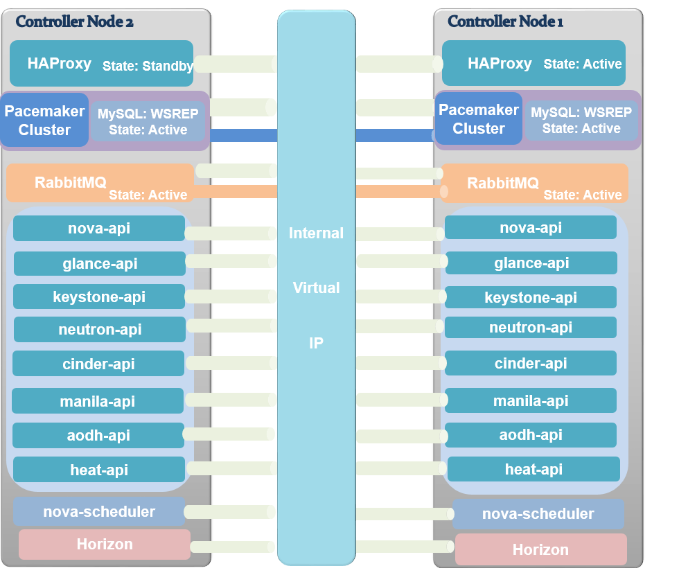
Obviously, in a highly available setup, we should achieve a degree of redundancy in each service within OpenStack. You may wonder about the critical OpenStack services claimed in the first part of this chapter: the database and message queue. Why can't they be separately clustered or packaged on their own? This is a pertinent question. Remember that we are still in the second logical phase where we try to dive slowly into the infrastructure without getting into the details. Besides, we keep on going from a generic and simple design to targeting specific use-cases. Decoupling infrastructure components such as RabbitMQ or MySQL from now on may lead to skipping the requirements of a simple design.
What about high availability?
The previous figure includes several essential solutions for a highly-scalable and redundant OpenStack environment such as virtual IP (VIP), HAProxy, and Pacemaker. The aforementioned technologies will be discussed in more detail in Chapter 9, Openstack HA and Failover.
The previous figure includes several essential solutions for a highly-scalable and redundant OpenStack environment such as virtual IP (VIP), HAProxy, and Pacemaker. The aforementioned technologies will be discussed in more detail in Chapter 9, Openstack HA and Failover.
Compute nodes are relatively simple as they are intended just to run the virtual machine's workload. In order to manage the VMs, the nova-compute service can be assigned for each compute node. Besides, we should not forget that the compute nodes will not be isolated; a Neutron agent and an optional Ceilometer compute agent may run these nodes.
Network nodes will run Neutron agents for DHCP, and L3 connectivity.
What about storage?
You should now have a deeper understanding of the storage types within Swift, Cinder, and Manila.
However, we have not covered third-party software-defined storage, Swift and Cinder.
More details will be covered in Chapter 5, OpenStack Storage , and File Share. For now, we will design from a basis where we have to decide how Cinder, Manila, and/or Swift will be a part of our logical design.
You will have to ask yourself questions such as: How much data do I need to store? Will my future use cases result in a wide range of applications that run heavy-analysis data? What are my storage requirements for incrementally backing up a virtual machine's snapshots? Do I really need control over the filesystem on the storage or is just a file share enough? Do I need a shared storage between VMs?
Many will ask the following question: If one can be satisfied by ephemeral storage, why offer block/share storage? To answer this question, you can think about ephemeral storage as the place where the end user will not be able to access the virtual disk associated with its VM when it is terminated. Ephemeral storage should mainly be used in production when the VM state is non-critical, where users or application don't store data on the VM. If you need your data to be persistent, you must plan for a storage service such as Cinder or Manila.
Remember that the current design applies for medium to large infrastructures. Ephemeral storage can also be a choice for certain users; for example, when they consider building a test environment. Considering the same case for Swift, we claimed previously that object storage might be used to store machine images, but when do we use such a solution? Simply put, when you have a sufficient volume of critical data in your cloud environment and start to feel the need for replication and redundancy.
Networking needs
One of the most complicated services defined previously should be connected.
The logical networking design
OpenStack allows a wide ranging of configurations that variation, and tunneled networks such as GRE, VXLAN, and so on, with Neutron are not intuitively obvious from their appearance to be able to be implemented without fetching their use case in our design. Thus, this important step implies that you may differ between different network topologies because of the reasons behind why every choice was made and why it may work for a given use case.
OpenStack has moved from simplistic network features to more complicated ones, but of course the reason is that it offers more flexibility! This is why OpenStack is here. It brings as much flexibility as it can! Without taking any random network-related decisions, let's see which network modes are available. We will keep on filtering until we hit the first correct target topology:
| Network mode | Network Characteristics | Implementation |
| nova-network | Flat network design without tenant traffic isolation | nova-network Flat DHCP |
|
Isolated tenants traffic and predefined fixed private IP space size Limited number of tenant networks (4K VLANs limit) |
nova-network VLANManager | |
| Neutron |
Isolated tenants traffic Limited number of tenant networks (4K VLANs limit) |
Neutron VLAN |
|
Increased number of tenant networks Increased packet size Lower performance |
Neutron tunneled networking (GRE, VXLAN, and so on) |
The preceding table shows a simple differentiation between two different logical network designs for OpenStack. Every mode shows its own requirements: this is very important and should be taken into consideration before the deployment.
Arguing about our example choice, since we aim to deploy a very flexible, large-scale environment we will toggle the Neutron choice for networking management instead of nova-network.
Note that it is also possible to keep on going with nova-network, but you have to worry about any Single Point Of Failure (SPOF) in the infrastructure. The choice was made for Neutron, since we started from a basic network deployment. We will cover more advanced features in the subsequent chapters of this book.
We would like to exploit a major advantage of Neutron compared to nova-network, which is the virtualization of Layers 2 and 3 of the OSI network model.
Let's see how we can expose our logical network design. For performance reasons; it is highly recommended to implement a topology that can handle different types of traffic by using separated logical networks.
In this way, as your network grows, it will still be manageable in case a sudden bottleneck or an unexpected failure affects a segment.
Let us look at the different rate the OpenStack environment the OpenStack environment
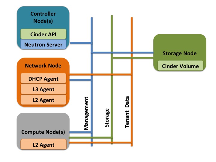
Physical network layout
We will start by looking at the physical networking requirements of the cloud.
The tenant data network
The main feature of a data network that it provides the physical path for the virtual networks created by the OpenStack tenants. It separates the tenant data traffic from the infrastructure communication path required for the communication between the OpenStack component itself.
Management and the API network
In a smaller deployment, the traffic for management and communication between the OpenStack components can be on the same physical link. This physical network provides a path for communication between the various OpenStack components such as REST API access and DB traffic, as well as for managing the OpenStack nodes.
For a production environment, the network can be further subdivided to provide better isolation of traffic and contain the load on the individual networks.
The Storage network
The storage network provides physical connectivity and isolation for storage-related traffic between the VMs and the storage servers. As the traffic load for the storage network is quite high, it is a good idea to isolate the storage network load from the management and tenant traffic.
Virtual Network types
Let's now look at the virtual network types and their features.
The external network
The features of an external or a public network are as follows:
- It provides global connectivity and uses routable IP addressing
- It is used by the virtual router to perform SNAT from the VM instances and provide external access to traffic originating from the VM and going to the Internet
SNAT refers to Source Network Address Translation. It allows traffic from a private network to go out to the Internet. OpenStack supports SNAT through its Neutron APIs for routers. More information can be found at http://en.wikipedia.org/wiki/Network_address_translation.
- It is used to provide a DNAT service for traffic from the Internet to reach a service running on the VM instance
While using VLANs, by tagging networks and combining multiple networks into one Network Interface Card (NIC), you can optionally leave the public network untagged for that NIC, to make the access to the OpenStack dashboard and the public OpenStack API endpoints simple.
The tenant networks
The features of the tenant network are as follows:
- It provides a private network between virtual machines
- It uses private IP space
- It provides isolation of tenant traffic and allows multi-tenancy requirements for networking services
The next step is to validate our network design in a simple diagram:
The physical model design
Finally, we will bring our logical design to life in the form of a physical design.
We can start with a limited number of servers just to setup the first deployment of our environment effectively.
You have to consider the fact that hardware commodity selection will accomplish the mission of our massive scalable architecture.
Estimating the hardware capabilities
Since the architecture is being designed to scale horizontally, we can add more servers to the setup. We will start by using commodity class, cost-effective hardware.
In order to expect our infrastructure economy, it would be great to make some basic hardware calculations for the first estimation of our exact requirements.
Considering the possibility of experiencing contentions for resources such as CPU, RAM, network, and disk, you cannot wait for a particular physical component to fail before you take corrective action, which might be more complicated.
Let's inspect a real-life example of the impact of underestimating capacity planning. A cloud-hosting company set up two medium servers, one for an e-mail server and the other to host the official website. The company, which is one of our several clients, grew in a few months and eventually ran out of disk space. The expected time to resolve such an issue is a few hours, but it took days. The problem was that all the parties did not make proper use of the cloud, due to the on demand nature of the service. This led to Mean Time To Repair (MTTR) increasing exponentially. The cloud provider did not expect this!
Incidents like this highlight the importance of proper capacity planning for your cloud infrastructure. Capacity management is considered a day-to-day responsibility where you have to stay updated with regard to software or hardware upgrades.
Through a continuous monitoring process of service consumption, you will be able to reduce the IT risk and provide a quick response to the customer's needs.
From your first hardware deployment, keep running your capacity management processes by looping through tuning, monitoring, and analysis.
The next stop will take into account your tuned parameters and introduce, within your hardware/software, the right change, which involves a synergy of the change management process.
Let's make our first calculation based on certain requirements. For example, let's say we aim to run 200 VMs in our OpenStack environment.
CPU calculations
The following are the calculation-related assumptions:
- 200 virtual machines
- No CPU oversubscribing
Processor over subscription is defined as the total number of CPUs that are assigned to all the powered-on virtual machines multiplied by the hardware CPU core. If this number is greater than the GHz purchased, the environment is oversubscribed.
- GHz per physical core = 2.6 GHz
- Physical core hyper-threading support = use factor 2
- GHz per VM (AVG compute units) = 2 GHz
- GHz per VM (MAX compute units) = 16 GHz
- Intel Xeon E5-2648L v2 core CPU = 10
- CPU sockets per server = 2
The formula for calculating the total number of CPU cores is as follows:
(number of VMs x number of GHz per VM) / number of GHz per core
(200 * 2) / 2.6 = 153.846
We have 153 CPU cores for 200 VMs.
The formula for calculating the number of core CPU sockets is as follows:
Total number of sockets / number of sockets per server
153 / 10 = 15.3
We will need 15 sockets
The formula for calculating the number of socket servers is as follows:
Total number of sockets / Number of sockets per server
15 / 2 = 7.5
You will need around seven to eight dual socket servers.
The number of virtual machines per server with eight dual socket servers is calculated as follows:
We can deploy 25 virtual machines per server
200 / 8 = 25
Number of virtual machines / number of servers
Memory calculations
Based on the previous example, 25 VMs can be deployed per compute node. Memory sizing is also important to avoid making unreasonable resource allocations.
Let's make an assumption list (keep in mind that it always depends on your budget and needs):
- 2 GB RAM per VM
- 8 GB RAM maximum dynamic allocations per VM
- Compute nodes supporting slots of: 2, 4, 8, and 16 GB sticks
- RAM available per compute node:
8 * 25 = 200 GB
Considering the number of sticks supported by your server, you will need around 256 GB installed. Therefore, the total number of RAM sticks installed can be calculated in the following way:
Total available RAM / MAX Available RAM-Stick size
256 / 16 = 16
Network calculations
To fulfill the plans that were drawn for reference, let's have a look at our assumptions:
- 200 Mbits/second is needed per VM
- Minimum network latency
To do this, it might be possible to serve our VMs by using a 10 GB link for each server, which will give:
10,000 Mbits/second / 25VMs = 400 Mbits/second
This is a very satisfying value. We need to consider another factor: highly available network architecture. Thus, an alternative is using two data switches with a minimum of 24 ports for data.
Thinking about growth from now, two 48-port switches will be in place.
What about the growth of the rack size? In this case, you should think about the example of switch aggregation that uses the Multi-Chassis Link Aggregation (MCLAG/MLAG) technology between the switches in the aggregation. This feature allows each server rack to divide its links between the pair of switches to achieve a powerful active-active forwarding while using the full bandwidth capability with no requirement for a spanning tree.
MCLAG is a Layer 2 link aggregation protocol between the servers that are connected to the switches, offering a redundant, load-balancing connection to the core network and replacing the spanning-tree protocol.
The network configuration also depends heavily on the chosen network topology. As shown in the previous example network diagram, you should be aware that all nodes in the OpenStack environment must communicate with each other. Based on this requirement, administrators will need to standardize the units will be planned to use and count the needed number of public and floating IP addresses. This calculation depends on which network type the OpenStack environment will run including the usage of Neutron or former nova-network service. It is crucial to separate which OpenStack units will need an attribution of Public and floating IPs. Our first basic example assumes the usage of the Public IPs for the following units:
- Cloud Controller Nodes: 3
- Compute Nodes: 15
- Storage Nodes: 5
In this case, we will initially need at least 18 public IP addresses. Moreover, when implementing a high available setup using virtual IPs fronted by load balancers, these will be considered as additional public IP addresses.
The use of Neutron for our OpenStack network design will involve a preparation for the number of virtual devices and interfaces interacting with the network node and the rest of the private cloud environment including:
- Virtual routers for 20 tenants: 20
- Virtual machines in 15 Compute Nodes: 375
In this case, we will initially need at least 395 floating IP addresses given that every virtual router is capable of connecting to the public network.
Additionally, increasing the available bandwidth should be taken into consideration in advance. For this purpose, we will need to consider the use of NIC bonding, therefore multiplying the number of NICs by 2. Bonding will empower cloud network high availability and achieve boosted bandwidth performance.
Storage calculations
Considering the previous example, you need to plan for an initial storage capacity per server that will serve 25 VMs each.
A simple calculation, assuming 100 GB ephemeral storage per VM, will require a space of 25*100 = 2.5 TB of local storage on each compute node.
You can assign 250 GB of persistent storage per VM to have 25*250 = 5 TB of persistent storage per compute node.
Most probably, you have an idea about the replication of object storage in OpenStack, which implies the usage of three times the required space for replication.
In other words, if you are planning for X TB for object storage, your storage requirement will be 3X.
Other considerations, such as the best storage performance using SSD, can be useful for a better throughput where you can invest more boxes to get an increased IOPS.
For example, working with SSD with 20K IOPS installed in a server with eight slot drives will bring you:
(20K * 8) / 25 = 6.4 K Read IOPS and 3.2K Write IOPS
That is not bad for a production starter!
Best practices
Well, let's bring some best practices under the microscope by exposing the OpenStack design flavor.
In a typical OpenStack production environment, the minimum requirement for disk space per compute node is 300 GB with a minimum RAM of 128 GB and a dual 8-core CPU.
Let's imagine a scenario where, due to budget limitations, you start your first compute node with costly hardware that has 600 GB disk space, 16-core CPUs, and 256 GB of RAM.
Assuming that your OpenStack environment continues to grow, you may decide to purchase more hardware: large, and at an incredible price! A second compute instance is placed to scale up.
Shortly after this, you may find out that demand is increasing. You may start splitting requests into different compute nodes but keep on continuing scaling up with the hardware. At some point, you will be alerted about reaching your budget limit!
There are certainly times when the best practices aren't in fact the best for your design. The previous example illustrated a commonly overlooked requirement for the OpenStack deployment.
If the minimal hardware requirement is strictly followed, it may result in an exponential cost with regards to hardware expenses, especially for new project starters.
Thus, you should choose exactly what works for you and consider the constraints that exist in your environment.
Keep in mind that best practices are a guideline; apply them when you find what you need to be deployed and how it should be set up.
On the other hand, do not stick to values, but stick to the spirit of the rules. Let's bring the previous example under the microscope again: scaling up shows more risk and may lead to failure than scaling out or horizontally. The reason behind such a design is to allow for a fast scale of transactions at the cost of duplicated compute functionality and smaller systems at a lower cost. That is how OpenStack was designed: degraded units can be discarded and failed workloads can be replaced.
Transactions and requests in the compute node may grow tremendously in a short time to a point where a single big compute node with 16 core CPUs starts failing performance-wise, while a few small compute nodes with 4 core CPUs can proceed to complete the job successfully.
As we have shown in the previous section, planning for capacity is a quite intensive exercise but very crucial to setting up an initial, successful OpenStack cloud strategy.
Planning for growth should be driven by the natural design of OpenStack and how it is implemented. We should consider that growth is based on demand where workloads in OpenStack take an elastic form and not a linear one. Although the previous resource's computation example can be helpful to estimate a few initial requirements for our designed OpenStack layout, reaching acceptable capacity planning still needs more action. This includes a detailed analysis of cloud performance in terms of growth of workload. In addition, by using more sophisticated monitoring tools, operators should be consistent in tracking the usage of each unit running in the OpenStack environment, which includes, for example, its overall resource consumption over time and cases of unit overutilization resulting in performance degradation. As we have conducted a rough estimation of our future hardware capabilities, this calculation model can be hardened by sizing the instance flavor for each compute host after first deployment and can be adjusted on demand if resources are carefully monitored.