Recall that a network's density is the number of actual edges versus the number of possible edges. A completely dense network is one that has an edge between each vertex and every other vertex. For example, in the following figure, the graph on the upper-right section is completely dense. The graph in the lower-left section has a density factor of 0.5333.

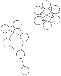
The number of possible edges is given as N(N-1). We'll define the density formula as follows:

(defn density [graph]
  (let [n (count (get-vertices graph))
        e (count (get-edges graph))]
    (/ (* 2.0 e) (* n (dec n)))))

We can use this to get some information about the number of edges in the graph:

user=> (g/density graph)
0.021504657198130255

Looking at this, it appears that this graph is not very dense. Maybe some other metrics will help explain why.

A vertex's degree is the number of other vertexes connected to it, and another summary statistic for social networks is the average degree. This is computed by the formula 2E/N. The Clojure to implement this is straightforward:

(defn avg-degree [graph]
  (/ (* 2.0 (count (get-edges graph)))
     (count (get-vertices graph))))

Similarly, it is easy to use it:

user=> (g/avg-degree graph)
85.11543319019954

So, the typical number of edges is around 85. Given that there are almost 4,000 vertices, it is understandable why the density is so low (0.022).

We can get a number of interesting metrics based on all of the paths between two elements. For example, we'll need those paths to get the centrality of nodes later in this chapter. The average path length is also an important metric. To calculate any of these, we'll need to compute all of the paths between any two vertices.

For weighted graphs that have a weight or cost assigned to each edge, there are a number of algorithms to find the shortest path. Dijkstra's algorithm and Johnson's algorithm are two common ones that perform well in a range of circumstances.

However, for non-weighted graphs, any of these search algorithms evolve into a breadth-first search. We just implemented this.

We can find the paths that use the breadth-first function that we walked through earlier. We simply take each vertex as a starting point and get all the paths from there. To make access easier later, we convert each path returned into a hash map as follows:

(defn find-all-paths [graph]
  (->> graph
    get-vertices
    (mapcat #(breadth-first graph %))
    (map #(hash-map :start (first %) :dest (last %) :path %))))

Unfortunately, there's an added complication; the output will probably take more memory than available. Because of this, we'll also define a couple of functions to write the paths out to a file and iterate over them again. We'll name them network-six.graph/write-paths and network-six.graph/iter-paths, and you can find them in the code download provided for this chapter on the Packt Publishing website. I saved it to the file path.json, as each line of the file is a separate JSON document.

The first metric that we can get from the paths is the average path length. We can find this easily by walking over the paths. We'll use a slightly different definition of mean that doesn't require all the data to be kept in the memory. You can find this in the network-six.util namespace:

user=> (double
         (u/mean
           (map count (map :path (g/iter-paths "path.json")))))
6.525055748717483

This is interesting! Strictly speaking, the concept of six degrees of separation says that all paths in the network should be six or smaller However, experiments often look at the paths in terms of the average path length. In this case, the average distance between any two connected nodes in this graph is just over six. So, the six degrees of separation do appear to hold in this graph.

We can see the distribution of path lengths more clearly by looking at a histogram of them:

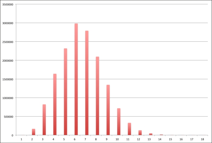
So, the distribution of path lengths appears to be more or less normal, centered on 6.

The network diameter is the longest of the shortest paths between any two nodes in the graph. This is simple to get:

user=> (reduce
         max Integer/MIN_VALUE
         (map count (map :path (g/iter-paths "path.json"))))
18

So the network diameter is approximately three times larger than the average.

Clustering coefficient is a measure of how many densely linked clusters there are in the graph. This is one measure of the small world effect, and it's sometimes referred to as the "all my friends know each other" property. To find the clustering coefficient for one vertex, this basically cuts all of its neighbors out of the network and tries to find the density of the subgraph. In looking at the whole graph, a high clustering coefficient indicates a small world effect in the graph.

The following is how to find the clustering coefficient for a single vertex:

(defn clustering-coeff [graph n]
  (let [cluster ((:neighbors graph) n)
        edges (filter cluster (mapcat (:neighbors graph) cluster))
        e (count edges)
        k (count cluster)]
    (if (= k 1)
      0
      (/ (* 2.0 e) (* k (dec k))))))

The function to find the average clustering coefficient for the graph is straightforward, and you can find it in the code download. The following is how it looks when applied to this graph:

user=> (g/avg-cluster-coeff graph)
1.0874536731229358

So it's not overly large. Chances are, there are a few nodes that are highly connected throughout the graph and most others are less connected.

There are several ways to measure how central a vertex is to the graph. One is closeness centrality. This is the distance of any particular vertex from all other vertices. We can easily get this information with the breadth-first function that we created earlier. Unfortunately, this only applies to complete networks, that is, to networks in which every vertex is reachable from every other vertex. This is not the case in the graph we're working with right now. There are some small pockets that are completely isolated from the rest of the network.

However, there are other measures of centrality that we can use instead. Betweenness centrality counts the number of shortest paths that a vertex is found in. Betweenness finds the vertices that act as a bridge. The original intent of this metric was to identify people who control the communication in the network.

To get this done efficiently, we can rely on the paths returned by the breadth-first function again. We'll get the paths from each vertex and call reduce over each. At every step, we'll calculate the total number of paths plus the number of times each vertex appears in a path:

(defn accum-betweenness
  [{:keys [paths betweenness reachable]} [v v-paths]]
  (let [v-paths (filter #(> (count %) 1) v-paths)]
    {:paths (+ paths (count v-paths)),
     :betweenness (merge-with +
                              betweenness
                              (frequencies (flatten v-paths))),
     :reachable (assoc reachable v (count v-paths))}))

Next, once we reach the end, we'll take the total number of paths and convert the betweenness and reachable totals for each vertex to a ratio, as follows:

(defn ->ratio [total [k c]]
  [k (double (/ c total))])
(defn finish-betweenness
  [{:keys [paths betweenness reachable] :as metrics}]
  (assoc metrics
         :betweenness (->> betweenness
                        (map #(->ratio paths %))
                        (into {}))
         :reachable (->> reachable
                      (map #(->ratio paths %))
                      (into {}))))

While these two functions do all the work, they aren't the public interface. The function metrics tie these two together in something we'd want to actually call:

(defn metrics [graph]
  (let [mzero {:paths 0, :betweenness {}, :reachable {}}]
    (->> graph
      get-vertices
      (pmap #(vector % (breadth-first graph %)))
      (reduce accum-betweenness mzero)
      finish-betweenness)))

We can now use this to find the betweenness centrality of any vertex as follows:

user=> (def m (g/metrics graph))
user=> ((:betweenness m) 0)
5.092923145895773E-4

Or, we can sort the vertices on the centrality measure to get those vertices that have the highest values. The first number in each pair of values that are returned is the node, and the second number is the betweenness centrality of that node. So, the first result says that the betweenness centrality for node 1085 is 0.254:

user=> (take 5 (reverse (sort-by second (seq (:betweenness m)))))
([1085 0.2541568423150047] [1718 0.1508391907570839] [1577 0.1228894724115601] [698 0.09236806137867479] [1505 0.08172539570689669])

This has all been interesting, but what about Kevin Bacon?

We started this chapter talking about the Six Degrees of Kevin Bacon, a pop culture phenomenon and how this captures a fundamental nature of many social networks. Let's analyze our Facebook network for this.

First, we'll create a function called degrees-between. This will take an origin vertex and a degree of separation to go out, and it will return a list of each level of separation and the vertices at that distance from the origin vertex. The degrees-between function will do this by accumulating a list of vertices at each level and a set of vertices that we've seen. At each step, it will take the last level and find all of those vertices' neighbors, without the ones we've already visited. The following is what this will look like:

(defn degrees-between [graph n from]
  (let [neighbors (:neighbors graph)]
    (loop [d [{:degree 0, :neighbors #{from}}],
           seen #{from}]
      (let [{:keys [degree neighbors]} (last d)]
        (if (= degree n)
          d
          (let [next-neighbors (->> neighbors
                             (mapcat (:neighbors graph))
                             (remove seen)
                             set)]
          (recur (conj d {:degree (inc degree)
                            :neighbors next-neighbors})
                   (into seen next-neighbors))))))))

Earlier, we included a way to associate data with a vertex, but we haven't used this yet. Let's exercise that feature to store the degrees of separation from the origin vertex in the graph. We can either call this function with the output of degrees-between or with the parameters to degrees-between:

(defn store-degrees-between
  ([graph degrees]
   (let [store (fn [g {:keys [degree neighbors]}]
                 (reduce #(set-value %1 %2 degree) g neighbors))]
     (reduce store graph degrees)))
  ([graph n from]
   (store-degrees-between graph (degrees-between graph n from))))

Finally, the full graph is a little large, especially for many visualizations. So, let's include a function that will let us zoom in on the graph identified by the degrees-between function. It will return both the original graph, with the vertex data fields populated and the subgraph of vertices within the n levels of separation from the origin vertex:

(defn degrees-between-subgraph [graph n from]
  (let [marked (store-degrees-between graph n from)
        v-set (set (map first (filter second (:data marked))))
        sub (subgraph marked v-set)]
    {:graph marked, :subgraph sub}))

With these defined, we can learn some more interesting things about the network that we're studying. Let's see how much of the network with different vertices can reach within six hops. Let's look at how we'd do this with vertex 0, and then we can see a table that presents these values for several vertices:

user=> (def v-count (count (g/get-vertices g)))
#'user/v-count
user=> (double
         (/ (count
              (g/get-vertices
                (:subgraph (g/degrees-between-subgraph g 6 0))))
            v-count))
0.8949229603435211

Now, it's interesting to see how the betweenness values for these track the amount of the graph that they can access quickly:

These are some interesting data points. What does this look like for the network as a whole?

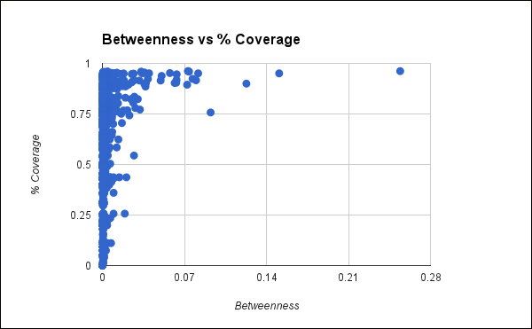
This makes it clear that there's probably little correlation between these two variables. Most vertices have a very low betweenness, although they range between 0 and 100 in the percent of the network that they can access.

At this point, we have some interesting facts about the network, but it would be helpful to get a more intuitive overview of it, like we just did for the betweenness centrality. Visualizations can help here.