
This final section introduces the key elements of the training and classification workflow. A test case using a simple logistic regression is used to illustrate each step of the computational workflow.
In its simplest form, a computational workflow to perform runtime processing of a dataset is composed of the following stages:
Loading the dataset from files, databases, or any streaming devices.
Splitting the dataset for parallel data processing.
Preprocessing data using filtering techniques, analysis of variance, and applying penalty and normalization functions whenever necessary.
Applying the model—either a set of clusters or classes—to classify new data.
Assessing the quality of the model.
A similar sequence of tasks is used to extract a model from a training dataset:
Loading the dataset from files, databases, or any streaming devices.
Splitting the dataset for parallel data processing.
Applying filtering techniques, analysis of variance, and penalty and normalization functions to the raw dataset whenever necessary.
Selecting the training, testing, and validation set from the cleansed input data.
Extracting key features and establishing affinity between a similar group of observations using clustering techniques or supervised learning algorithms.
Reducing the number of features to a manageable set of attributes to avoid overfitting the training set.
Validating the model and tuning the model by iterating steps 5, 6, and 7 until the error meets a predefined convergence criteria.
Storing the model in a file or database so that it can be applied to future observations.
Data clustering and data classification can be performed independent of each other or as part of a workflow that uses clustering techniques at the preprocessing stage of the training phase of a supervised learning algorithm. Data clustering does not require a model to be extracted from a training set, while classification can be performed only if a model has been built from the training set. The following image gives an overview of training, classification, and validation:
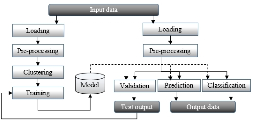
A generic data flow for training and running a model
The preceding diagram is an overview of a typical data mining processing pipeline. The first phase consists of extracting the model through clustering or training of a supervised learning algorithm. The model is then validated against test data for which the source is the same as the training set but with different observations. Once the model is created and validated, it can be used to classify real-time data or predict future behavior. Real-world workflows are more complex and require dynamic configuration to allow experimentation of different models. Several alternative classifiers can be used to perform a regression and different filtering algorithms are applied against input data, depending on the latent noise in the raw data.
This book relies on financial data to experiment with different learning strategies. The objective of the exercise is to build a model that can discriminate between volatile and nonvolatile trading sessions for stock or commodities. For the first example, we select a simplified version of the binomial logistic regression as our classifier as we treat stock-price-volume action as a continuous or pseudo-continuous process.
Note
An introduction to the logistic regression
Logistic regression is explained in depth in the Logistic regression section in Chapter 6, Regression and Regularization. The model treated in this example is the simple binomial logistic regression classifier for two-dimension observations.
The steps for classification of trading sessions according to their volatility and volume is as follows:
Scoping the problem
Loading data
Preprocessing raw data
Discovering patterns, whenever possible
Implementing the classifier
Evaluating the model
The objective is to create a model for stock price using its daily trading volume and volatility. Throughout the book, we will rely on financial data to evaluate and discuss the merits of different data processing and machine learning methods. In this example, the data is extracted from Yahoo Finances using the CSV format with the following fields:
Date
Price at open
Highest price in the session
Lowest price in the session
Price at session close
Volume
Adjust price at session close
The YahooFinancials enumerator extracts the historical daily trading information from the Yahoo finance site:
type Fields = Array[String]
object YahooFinancials extends Enumeration {
   type YahooFinancials = Value
   val DATE, OPEN, HIGH, LOW, CLOSE, VOLUME, ADJ_CLOSE = Value

   def toDouble(v: Value): Fields => Double =   //1
   (s: Fields) => s(v.id).toDouble
   def toDblArray(vs: Array[Value]): Fields => DblArray = //2
       (s: Fields) => vs.map(v => s(v.id).toDouble)
  …
}
The toDouble method converts an array of string into a single value (line 1) and toDblArray converts an array of string into an array of values (line 2). The YahooFinancials enumerator is described in the Data sources section in Appendix A, Basic Concepts in detail.
Let's create a simple program that loads the content of the file, executes some simple preprocessing functions, and creates a simple model. We selected the CSCO stock price between January 1, 2012 and December 1, 2013 as our data input.
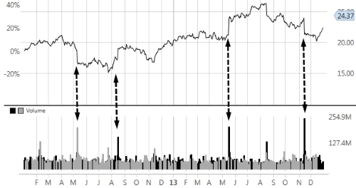
Let's consider the two variables, price and volume, as shown in the following screenshot. The top graph displays the variation of the price of Cisco stock over time and the bottom bar chart represents the daily trading volume on Cisco stock over time:
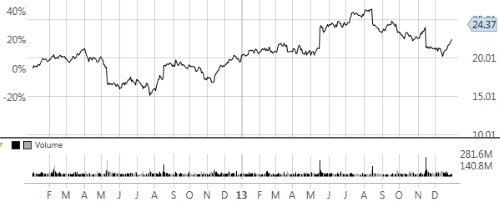
Price-Volume action for Cisco stock 2012-2013
The second step is loading the dataset from a local or remote data storage. Typically, large datasets are loaded from a database or distributed filesystems such as Hadoop Distributed File System (HDFS). The load method takes an absolute pathname, extract, and transforms the input data from a file into a time series of a Vector[DblPair] type:
def load(fileName: String): Try[Vector[DblPair]] = Try {
   val src =  Source.fromFile(fileName)  //3
   val data = extract(src.getLines.map(_.split(",")).drop(1)) //4
   src.close //5
   data
 }
The data file is extracted through an invocation of the Source.fromFile static method (line 3), and then the fields are extracted through a map before the header (first row in the file) is removed using drop (line 4). The file has to be closed to avoid leaking of the file handle (line 5).
Note
Data extraction
The Source.fromFile.getLines.map invocation pipeline method returns an iterator that can be traversed only once.
The purpose of the extract method is to generate a time series of two variables (relative stock volatility and relative stock daily trading volume):
def extract(cols: Iterator[Array[String]]): XVSeries[Double]= {
  val features = Array[YahooFinancials](LOW, HIGH, VOLUME) //6
  val conversion = YahooFinancials.toDblArray(features)  //7
  cols.map(c => conversion(c)).toVector
      .map(x => Array[Double](1.0 - x(0)/x(1), x(2)))  //8
}
The only purpose of the extract method is to convert the raw textual data into a two-dimensional time series. The first step consists of selecting the three features to extract LOW (the lowest stock price in the session), HIGH (the highest price in the session), and VOLUME (trading volume for the session) (line 6). This feature set is used to convert each line of fields into a corresponding set of three values (line 7). Finally, the feature set is reduced to the following two variables (line 8):
Relative volatility of the stock price in a session: 1.0 – LOW/HIGH
Trading volume for the stock in the session: VOLUME
Note
Code readability
A long pipeline of Scala high-order methods make the code and underlying code quite difficult to read. It is recommended that you break down long chains of method calls, such as the following:
val cols = Source.fromFile.getLines.map(_.split(",")).toArray.drop(1)We can break down method calls into several steps as follows:
val lines = Source.fromFile.getLines
val fields = lines.map(_.split(",")).toArray
val cols = fields.drop(1)
We strongly encourage you to consult the excellent guide Effective Scala, written by Marius Eriksen from Twitter. This is definitively a must read for any Scala developer [1:10].
The next step is to normalize the data in the range [0.0, 1.0] to be trained by the binomial logistic regression. It is time to introduce an immutable and flexible normalization class.
The logistic regression relies on the sigmoid curve or logistic function is described in the Logistic function section in Chapter 6, Regression and Regularization. The logistic functions are used to segregate training data into classes. The output value of the logistic function ranges from 0 for x = - INFINITY to 1 for x = + INFINITY. Therefore, it makes sense to normalize the input data or observation over [0, 1].
Note
Normalize or not normalize?
The purpose of normalizing data is to impose a single range of values for all the features, so the model does not favor any particular feature. Normalization techniques include linear normalization and Z-score. Normalization is an expensive operation that is not always needed.
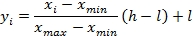
The normalization is a linear transformation of the raw data that can be generalized to any range [l, h].
Note
Linear normalization
M2: [0, 1] Normalization of features {xi} with minimum xmin and maximum xmax values:
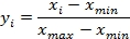
M3: [l, h] Normalization of features {xi}:
The normalization of input data in supervised learning has a specific requirement: the classification and prediction of new observations have to use the normalization parameters (min and max) extracted from the training set, so all the observations share the same scaling factor.
Let's define the MinMax normalization class. The class is immutable: the minimum, min, and maximum, max, values are computed within the constructor. The class takes a time series of a parameterized T type and values as arguments (line 8). The steps of the normalization process are defined as follows:
Initialize the minimum values for a given time series during instantiation (line
9).Compute the normalization parameters (line
10) and normalize the input data (line11).Normalize any new data points reusing the normalization parameters (line
14):class MinMax[T <: AnyVal](val values: XSeries[T]) (f : T => Double) { //8 val zero = (Double.MaxValue, -Double.MaxValue) val minMax = values./:(zero)((mM, x) => { //9 val min = mM._1 val max = mM._2 (if(x < min) x else min, if(x > max) x else max) }) case class ScaleFactors(low:Double ,high:Double, ratio: Double) var scaleFactors: Option[ScaleFactors] = None //10 def min = minMax._1 def max = minMax._2 def normalize(low: Double, high: Double): DblVector //11 def normalize(value: Double): Double }
The class constructor computes the tuple of minimum and maximum values, minMax, using a fold (line 9). The scaleFactors scaling parameters are computed during the normalization of the time series (line 11), which are described as follows. The normalize method initializes the scaling factor parameters (line 12) before normalizing the input data (line 13):
def normalize(low: Double, high: Double): DblVector =
  setScaleFactors(low, high).map( scale => { //12
    values.map(x =>(x - min)*scale.ratio + scale.low) //13
  }).getOrElse(/* … */)

def setScaleFactors(l: Double, h: Double): Option[ScaleFactors]={
    // .. error handling code
   Some(ScaleFactors(l, h, (h - l)/(max - min))
}
Subsequent observations use the same scaling factors extracted from the input time series in normalize (line 14):
def normalize(value: Double):Double = setScaleFactors.map(scale =>
   if(value < min) scale.low
   else if (value > max) scale.high
   else (value - min)* scale.high + scale.low
).getOrElse( /* … */)
The MinMax class normalizes single variable observations.
Note
The statistics class
The class that extracts the basic statistics from a Stats dataset, which is introduced in the Profiling data section in Chapter 2, Hello World!, inherits the MinMax class.
The test case with the binomial logistic regression uses a multiple variable normalization, implemented by the MinMaxVector class, which takes observations of the XVSeries[Double] type as inputs:
class MinMaxVector(series: XVSeries[Double]) {
  val minMaxVector: Vector[MinMax[Double]] = //15
      series.transpose.map(new MinMax[Double](_))
  def normalize(low: Double, high: Double): XVSeries[Double]
}
The constructor of the MinMaxVector class transposes the vector of array of observations in order to compute the minimum and maximum value for each dimension (line 15).
The price action chart has a very interesting characteristic.
At a closer look, a sudden change in price and increase in volume occurs about every three months or so. Experienced investors will undoubtedly recognize that these price-volume patterns are related to the release of quarterly earnings of Cisco. Such a regular but unpredictable pattern can be a source of concern or opportunity if risk can be properly managed. The strong reaction of the stock price to the release of corporate earnings may scare some long-term investors while enticing day traders.
The following graph visualizes the potential correlation between sudden price change (volatility) and heavy trading volume:
Price-volume correlation for the Cisco stock 2012-2013
The next section is not required for the understanding of the test case. It illustrates the capabilities of JFreeChart as a simple visualization and plotting library.
Although charting is not the primary goal of this book, we thought that you will benefit from a brief introduction to JFreeChart.
Note
Plotting classes
This section illustrates a simple Scala interface to JFreeChart Java classes. Reading this is not required for the understanding of machine learning. The visualization of the results of a computation is beyond the scope of this book.
Some of the classes used in visualization are described in the Appendix A, Basic Concepts.
The dataset (volatility and volume) is converted into internal JFreeChart data structures. The ScatterPlot class implements a simple configurable scatter plot with the following arguments:
config: This includes information, labels, fonts, and so on, of the plottheme: This is the predefined theme for the plot (black, white background, and so on)
The code will be as follows:
class ScatterPlot(config: PlotInfo, theme: PlotTheme) { //16
  def display(xy: Vector[DblPair], width: Int, height) //17
  def display(xt: XVSeries[Double], width: Int, height)
  // ….
}
The PlotTheme class defines a specific theme or preconfiguration of the chart (line 16). The class offers a set of display methods to accommodate a wide range of data structures and configuration (line 17).
Note
Visualization
The JFreeChart library is introduced as a robust charting tool. The code related to plots and charts is omitted from the book in order to keep the code snippets concise and dedicated to machine learning. On a few occasions, output data is formatted as a CSV file to be imported into a spreadsheet.
The ScatterPlot.display method is used to display the normalized input data used in the binomial logistic regression as follows:
val plot = new ScatterPlot(("CSCO 2012-2013",
   "Session High - Low", "Session Volume"), new BlackPlotTheme)
plot.display(volatility_vol, 250, 340)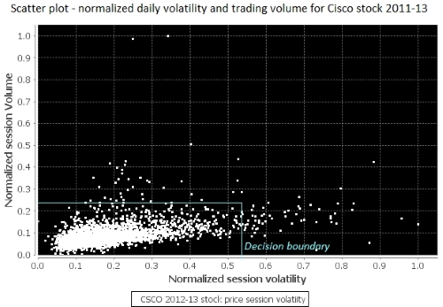
A scatter plot of volatility and volume for the Cisco stock 2012-2013
The scatter plot shows a level of correlation between session volume and session volatility and confirms the initial finding in the stock price and volume chart. We can leverage this information to classify trading sessions by their volatility and volume. The next step is to create a two class model by loading a training set, observations, and expected values, into our logistic regression algorithm. The classes are delimited by a decision boundary (also known as a hyperplane) drawn on the scatter plot.
Visualizing labels—the normalized variation of the stock price between the opening and closing of the trading session is selected as the label for this classifier.
The objective of this training is to build a model that can discriminate between volatile and nonvolatile trading sessions. For the sake of the exercise, session volatility is defined as the relative difference between the session highest price and lower price. The total trading volume within a session constitutes the second parameter of the model. The relative price movement within a trading session (that is, closing price/open price - 1) is our expected values or labels.
Logistic regression is commonly used in statistics inference.
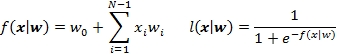
The first weight w0 is known as the intercept. The binomial logistic regression is described in the Logistic regression section in Chapter 6, Regression and Regularization, in detail.
The following implementation of the binomial logistic regression classifier exposes a single classify method to comply with our desire to reduce the complexity and life cycle of objects. The model weights parameters are computed during training when the LogBinRegression class/model is instantiated. As mentioned earlier, the sections of the code nonessential to the understanding of the algorithm are omitted.
The LogBinRegression constructor has five arguments (line 18):
The code is as follows:
class LogBinRegression(
     obsSet: Vector[DblArray],
     expected: Vector[Int],
     maxIters: Int,
     eta: Double,
     eps: Double) {  //18

   val model: LogBinRegressionModel = train  //19
   def classify(obs: DblArray): Try[(Int, Double)]   //20
   def train: LogBinRegressionModel
   def intercept(weights: DblArray): Double
   …
}
The LogBinRegressionModel model is generated through training during the instantiation of the LogBinRegression logistic regression class (line 19):
case class LogBinRegressionModel(val weights: DblArray)The model is fully defined by its weights, as described in the mathematical formula M3. The weights(0) intercept represents the mean value of the prediction for observations for which variables are zero. The intercept does not have any specific meaning for most of the cases and it is not always computable.
Note
Intercept or not intercept?
The intercept corresponds to the value of weights when the observations have null values. It is a common practice to estimate, whenever possible, the intercept for binomial linear or logistic regression independently from the slope of the model in the minimization of the error function. The multinomial regression models treat the intercept or weight w0 as part of the regression model, as described in the Ordinary least squares regression section of Chapter 6, Regression and Regularization.
The code will be as follows:
def intercept(weights: DblArray): Double = {
  val zeroObs = obsSet.filter(!_.exists( _ > 0.01))
  if( zeroObs.size > 0)
    zeroObs.aggregate(0.0)((s,z) => s + dot(z, weights),
       _ + _ )/zeroObs.size
  else 0.0
}
The classify methods takes new observations as inputs and compute the index of the classes (0 or 1) the observations belong to and the actual likelihood (line 20).
The goal of the training of a model using expected values is to compute the optimal weights that minimizes the error or cost function. We select the batch gradient descent algorithm to minimize the cumulative error between the predicted and expected values for all the observations. Although there are quite a few alternative optimizers, the gradient descent is quite robust and simple enough for this first chapter. The algorithm consists of updating the weights wi of the regression model by minimizing the cost.
Note
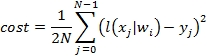
Cost function
M5: Cost (or compound error = predicted – expected):
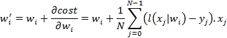
M6: The batch gradient descent method to update model weights wi is as follows:
For those interested in learning about of optimization techniques, the Summary of optimization techniques section in the Appendix A, Basic Concepts presents an overview of the most commonly used optimizers. The batch descent gradient method is also used for the training of the multilayer perceptron (refer to The training epoch section under The multilayer perceptron section in Chapter 9, Artificial Neural Networks).
The execution of the batch gradient descent algorithm follows these steps:
Initialize the weights of the regression model.
Shuffle the order of observations and expected values.
Aggregate the cost or error for the entire observation set.
Update the model weights using the cost as the objective function.
Repeat from step 2 until either the maximum number of iterations is reached or the incremental update of the cost is close to zero.
The purpose of shuffling the order of the observations between iterations is to avoid the minimization of the cost reaching a local minimum.
Tip
Batch and stochastic gradient descent
The stochastic gradient descent is a variant of the gradient descent that updates the model weights after computing the error on each observation. Although the stochastic gradient descent requires a higher computation effort to process each observation, it converges toward the optimal value of weights fairly quickly after a small number of iterations. However, the stochastic gradient descent is sensitive to the initial value of the weights and the selection of the learning rate, which is usually defined by an adaptive formula.
The train method consists of iterating through the computation of the weight using a simple descent gradient method. The method computes weights and returns an instance of the LogBinRegressionModel model:
def train: LogBinRegressionModel = {
  val nWeights = obsSet.head.length + 1  //21
  val init = Array.fill(nWeights)(Random.nextDouble )  //22
  val weights = gradientDescent(obsSet.zip(expected),0.0,0,init)
  new LogBinRegressionModel(weights)   //23
}
The train method extracts the number of weights, nWeights, for the regression model as the number of variables in each observation + 1 (line 21). The method initializes weights with random values over [0, 1] (line 22). The weights are computed through the tail recursive gradientDescent method, and the method returns a new model for the binomial logistic regression (line 23).
Tip
Unwrapping values from Try
It is usually not recommended to invoke the get method to a Try value, unless it is enclosed in a Try statement. The best course of action is to do the following:
1. Catch the failure with match{ case Success(m) => ..case Failure(e) =>}
2. Extract the getOrElse( /* … */ ) result safely
3. Propagate the results as a Try type map( _.m)
Let's take a look at the computation for weights through the minimization of the cost function in the gradientDescent method:
type LabelObs = Vector[(DblArray, Int)]

@tailrec
def gradientDescent(
      obsAndLbl: LabelObs,
      cost: Double,
      nIters: Int,
      weights: DblArray): DblArray = {  //24

  if(nIters >= maxIters)
       throw new IllegalStateException("..")//25
  val shuffled = shuffle(obsAndLbl)   //26
  val errorGrad = shuffled.map{ case(x, y) => {  //27
      val error = sigmoid(dot(x, weights)) - y
      (error, x.map( _ * error))  //28
   }}.unzip

   val scale = 0.5/obsAndLbl.size
   val newCost = errorGrad._1   //29
.aggregate(0.0)((s,c) =>s + c*c, _ + _ )*scale
   val relativeError = cost/newCost - 1.0

   if( Math.abs(relativeError) < eps)  weights  //30
   else {
     val derivatives = Vector[Double](1.0) ++
                 errorGrad._2.transpose.map(_.sum) //31
     val newWeights = weights.zip(derivatives)
                       .map{ case (w, df) => w - eta*df)  //32
     newWeights.copyToArray(weights)
     gradientDescent(shuffled, newCost, nIters+1, newWeights)//33
   }
}
The gradientDescent method recurses on the vector of pairs (observations and expected values), obsAndLbl, cost, and the model weights (line 24). It throws an exception if the maximum number of iterations allowed for the optimization is reached (line 25). It shuffles the order of the observations (line 26) before computing the errorGrad derivatives of the cost over each weights (line 27). The computation of the derivative of the cost (or error = predicted value – expected value) in formula M5 returns a pair of cumulative cost and derivative values using the formula (line 28).
Next, the method computes the overall compound cost using the formula M4 (line 29), converts it to a relative incremental relativeError cost that is compared to the eps convergence criteria (line 30). The method extracts derivatives of cost over weights by transposing the matrix of errors, and then prepends the bias 1.0 value to match the array of weights (line 31).
Note
Bias value
The purpose of the bias value is to prepend 1.0 to the vector of observation so it can be directly processed (for example, zip and dot) with the weights. For instance, a regression model for two-dimensional observations (x, y) has three weights (w0, w1, w2). The bias value +1 is prepended to the observations to compute the predicted value 1.0: w0 + x.w1, +
y.w2.
This technique is used in the computation of the activation function of the multilayer perceptron, as described in the The multilayer perceptron section in Chapter 9, Artificial Neural Networks.
The formula M6 updates the weights for the next iteration (line 32) before invoking the method with new weights, cost, and iteration count (line 33).
Let's take a look at the shuffling of the order of observations using a random sequence generator. The following implementation is an alternative to the Scala standard library method scala.util.Random.shuffle for shuffling elements of collections. The purpose is to change the order of observations and labels between iterations in order to prevent the optimizer to reach a local minimum. The shuffle method permutes the order in the labelObs vector of observations by partitioning it into segments of random size and reversing the order of the other segment:
val SPAN = 5
def shuffle(labelObs: LabelObs): LabelObs = {
  shuffle(new ArrayBuffer[Int],0,0).map(labelObs( _ )) //34
}
Once the order of the observations is updated, the vector of pair (observations, labels) is easily built through a map (line 34). The actual shuffling of the index is performed in the following shuffle recursive function:
val maxChunkSize = Random.nextInt(SPAN)+2  //35

@tailrec
def shuffle(indices: ArrayBuffer[Int], count: Int, start: Int):
      Array[Int] = {
  val end = start + Random.nextInt(maxChunkSize) //36
  val isOdd = ((count & 0x01) != 0x01)
  if(end >= sz)
    indices.toArray ++ slice(isOdd, start, sz) //37
  else
    shuffle(indices ++ slice(isOdd, start, end), count+1, end)
}
The maximum size of partition of the maxChunkSize vector observations is randomly computed (line 35). The method extracts the next slice (start, end) (line 36). The slice is either added to the existing indices vector and returned once all the observations have been shuffled (line 37) or passed to the next invocation.
The slice method returns an array of indices over the range (start, end) either in the right order if the number of segments processed is odd, or in reverse order if the number of segment processed is even:
def slice(isOdd: Boolean, start: Int, end: Int): Array[Int] = {
  val r = Range(start, end).toArray
  (if(isOdd) r else r.reverse)
}
Note
Iterative versus tail recursive computation
The tail recursion in Scala is a very efficient alternative to the iterative algorithm. Tail recursion avoids the need to create a new stack frame for each invocation of the method. It is applied to the implementation of many machine learning algorithms presented throughout the book.
In order to train the model, we need to label the input data. The labeling process consists of associating the relative price movement during a session (price at close/price at open – 1) with one of the following two configurations:
Volatile trading sessions with high trading volume
Trading sessions with low volatility and low trading volume
The two classes of training observations are segregated by a decision boundary drawn on the scatter plot in the previous section. The labeling process is usually quite cumbersome and should be automated as much as possible.
Once the model is successfully created through training, it is available to classify new observation. The runtime classification of observations using the binomial logistic regression is implemented by the classify method:
def classify(obs: DblArray): Try[(Int, Double)] =
  val linear = dot(obs, model.weights)  //37
  val prediction = sigmoid(linear)
  (if(linear > 0.0) 1 else 0, prediction) //38
})
The method applies the logistic function to the linear inner product, linear, of the new obs and weights observations of the model (line 37). The method returns the tuple (the predicted class of the observation {0, 1}, prediction value) where the class is defined by comparing the prediction to the boundary value 0.0 (line 38).
The computation of the dot product of weights and observations uses the bias value as follows:
def dot(obs: DblArray, weights: DblArray): Double =
   weights.zip(Array[Double](1.0) ++ obs)
          .aggregate(0.0){case (s, (w,x)) => s + w*x, _ + _ }
The alternative implementation of the dot product of weights and observations consists of extracting the first w.head weight:
def dot(x: DblArray, w: DblArray): Double =
  x.zip(w.drop(1)).map {case (_x,_w) => _x*_w}.sum + w.head
The dot method is used in the classify method.
The first step is to define the configuration parameters for the test: the maximum number of NITERS iterations, the EPS convergence criteria, the ETA learning rate, the decision boundary used to label the BOUNDARY training observations, and the path to the training and test sets:
val NITERS = 800; val EPS = 0.02; val ETA = 0.0001
val path_training = "resources/data/chap1/CSCO.csv"
val path_test = "resources/data/chap1/CSCO2.csv"
The various activities of creating and testing the model, loading, normalizing data, training the model, loading, and classifying test data is organized as a workflow using the monadic composition of the Try class:
for {
  volatilityVol <- load(path_training)    //39
  minMaxVec <- Try(new MinMaxVector(volatilityVol))    //40
  normVolatilityVol <- Try(minMaxVec.normalize(0.0,1.0))//41
  classifier <- logRegr(normVolatilityVol)    //42
  testValues <- load(path_test)    //43
  normTestValue0 <- minMaxVec.normalize(testValues(0))  //44
  class0 <- classifier.classify(normTestValue0)   //45
  normTestValue1 <- minMaxVec.normalize(testValues(1))
  class1 <- classifier.classify(normTestValues1)
} yield {
   val modelStr = model.toString
   …
}
First, the daily trading volatility and volume for the volatilityVol stock price is loaded from file (line 39). The workflow initializes the multi-dimensional MinMaxVec normalizer (line 40) and uses it to normalize the training set (line 41). The logRegr method instantiates the binomial classifier logistic regression (line 42). The testValues test data is loaded from file (line 43), normalized using MinMaxVec already applied to the training data (line 44), and classified (line 45).
The load method extracts data (observations) of a XVSeries[Double] type from the file. The heavy lifting is done by the extract method (line 46), and then the file handle is closed (line 47) before returning the vector of raw observations:
def load(fileName: String): Try[XVSeries[Double], XSeries[Double]] =  {
  val src =  Source.fromFile(fileName)
  val data = extract(src.getLines.map( _.split(",")).drop(1)) //46
  src.close; data //47
}
The private logRegr method has the following two purposes:
Labeling automatically the
obsobservations to generate theexpectedvalues (line48)Initializing (instantiation and training of the model) the binomial logistic regression (line
49)
The code is as follows:
def logRegr(obs: XVSeries[Double]): Try[LogBinRegression] = Try {
    val expected = normalize(labels._2).get  //48
    new LogBinRegression(obs, expected, NITERS, ETA, EPS)  //49
}
The method labels observations by evaluating if they belong to any one of the two classes delimited by the BOUNDARY condition, as illustrated in the scatter plot in a previous section.
Note
Validation
The simple classification in this test case is provided for illustrating the runtime application of the model. It does not constitute a validation of the model by any stretch of imagination. The next chapter digs into validation methodologies (refer to the Assessing a model section in Chapter 2, Hello World!
The training run is performed with three different values of the learning rate. The following chart illustrates the convergence of the batch gradient descent in the minimization of the cost, given different values of learning rates:
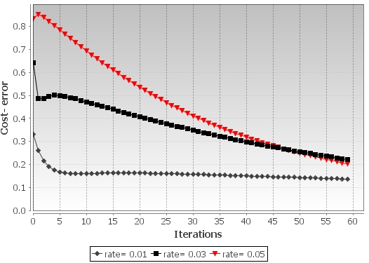
Impact of the learning rate on the batch gradient descent on the convergence of the cost (error)
As expected, the execution of the optimizer with a higher learning rate produces a steepest descent in the cost function.
The execution of the test produces the following model:
iters = 495
weights: 0.859-3.6177923,-64.927832
input (0.0088, 4.10E7) normalized (0.063,0.061) class 1 prediction 0.515
input (0.0694, 3.68E8) normalized (0.517,0.641) class 0 prediction 0.001
Note
Learning more about regressive models
The binomial logistic regression is merely used to illustrate the concept of training and prediction. It is described in the Logistic regression section in Chapter 6, Regression and Regularization in detail.