The phase when an algorithm runs over a labeled data set is known as training, and the labeled data is known as training dataset. Sometimes it is loosely referred to as training corpus. Later in the process, the algorithm must be tested with similar un-labeled datasets or for which the label is hidden from the algorithm. This dataset is known as test dataset or test corpus. Typically, an 80-20 split is used to generate the training and test set from a randomly shuffled labeled data set. This means that 80% of the randomly shuffled labeled data is generally treated as training data and the remaining 20% as test data.

Supervised learning algorithms have several applications. Following are some of those. This is by no means a comprehensive list, but it is indicative.

In the next few sections, I will walk you through the overview of a few of these algorithms and their mathematical basis. However, we will get away with as minimal math as possible, since the objective of the book is to help you use machine learning in the real settings.

As the name suggests, k-Nearest Neighbor is an algorithm that works on the distance between two projected points. It relies on the distance of k-nearest neighbors (thus the name) to determine the class/category of the unknown/new test data.

As the name suggests the nearest neighbor algorithm relies on the distance of two data points projected in N-Dimensional space. Let's take a popular example where the k-NN can be used to determine the class. The dataset https://archive.ics.uci.edu/ml/machine-learning-databases/breast-cancer-wisconsin/wdbc.data stores data about several patients who were either unfortunate and diagnosed as "Malignant" cases (which are represented as M in the dataset), or were fortunate and diagnosed as "Benign" (non-harmful/non-cancerous) cases (which are represented as B in the dataset). If you want to understand what all the other fields mean, take a look at https://archive.ics.uci.edu/ml/machine-learning-databases/breast-cancer-wisconsin/wdbc.names.

Now the question is, given a new entry with all the other records except the tag M or B, can we predict that? In ML terminology, this value "M" or "B" is sometimes referred to as "class tag" or just "class". The task of a classification algorithm is to determine this class for a new data point. K-NN does this in the following way: it measures the distance from the given data to all the training data and then takes into consideration the classes for only the k-nearest neighbors to determine the class of the new entry. So for the current case, if more than 50% of the k-nearest neighbors is of class "B", then k-NN will conclude that the new entry is of type "B".

The distance metric used is generally Euclidean, that you learnt in high school. For example, given two points in 3D.

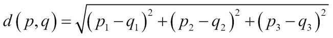
In this preceding example, and denote their values in the X axis, and denote their values in the Y axis, and and denote their values in the axis.

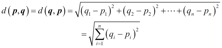
Extrapolating this, we get the following formula for calculating the distance in N dimension:

Thus, after calculating the distance from all the training set data, we can create a list of tuples with the distance and the class, as follows. This list is made for the sake of demonstration. This is not calculated from the actual data.

Let's assume that k is set to be 4. Now for each k, we take into consideration the class. So for the first three entries, we found that the class is B and for the last one, it is M. Since the number of B's is more than the number of M's, k-NN will conclude that the new patient's data is of type B.

Have you ever played the game where you had to guess about a thing that your friend had been thinking about by asking questions? And you were allowed to guess only a certain number of times and had to get back to your friend with your answer about what he/she could probably be thinking about.

The strategy to guess the correct answer is to start asking questions that segregate the possible answer space as evenly as possible. For example, if your friend told you that he/she had imagined about something, then probably the first question you would like to ask him/her is that whether he/she is thinking about an animal or a thing. That would broadly classify the answer space and then later you can ask more direct/specific questions based on the answers previously provided by your friend.

Decision tree is a set of classification algorithm that uses this approach to determine the class of an unknown entry. As the name suggests, a decision tree is a tree where the nodes depict the questions asked and the edges represent the decisions (yes/no). Leaf nodes determine the final class of the unknown entry. Following is a classic textbook example of a decision tree:

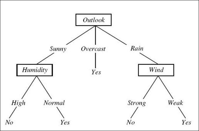
The preceding figure depicts the decision whether we can play lawn tennis or not, based on several attributes such as Outlook, Humidity, and Wind. Now the question that you may have is why outlook was chosen as the root node of the tree. The reason was that by choosing outlook as the first feature/attribute to split the dataset, the outcomes were split more evenly than if the split had been done with other attributes such as "humidity" or "wind".

The process of finding the attribute that can split the dataset more evenly than others is guided by entropy. Lesser the entropy, better the parameter. Entropy is known as the measure of information gain. It is calculated by the following formula:

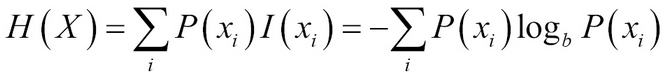
Here stands for the probability of and denotes the information gain.

Let's take the example of tennis dataset from Weka. Following is the file in the CSV format:

outlook,temperature,humidity,wind,playTennis
sunny, hot, high, weak, no
sunny, hot, high, strong, no
overcast, hot, high, weak, yes
rain, mild, high, weak, yes
rain,cool, normal, weak, yes
rain, cool, normal, strong, no
overcast, cool, normal, strong, yes
sunny, mild, high, weak, no
sunny, cool, normal, weak, yes
rain, mild, normal, weak, yes
sunny, mild, normal, strong, yes
overcast, mild, high, strong, yes
overcast, hot, normal, weak, yes
rain, mild, high, strong, no

You can see from the dataset that out of 14 instances (there are 14 rows in the file), 5 instances had the value no for playTennis and 9 instances had the value yes. Thus, the overall information is given by the following formula:

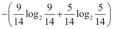
This roughly evaluates to 0.94. Now from the next steps, we must pick the attribute that maximizes the information gain. Information gain is denoted as the difference between the total entropy and the entropy calculated for each possible split.

Let's go with one example. For the outlook attribute, there are three possible values: rain, sunny, and overcast, and for each of these values, the value of the attribute playTennis is either no or yes.

For rain, out of 5 instances, 3 instances have the value yes for the attribute playTennis; thus, the entropy is as follows:

This is equal to 0.97.

For overcast, every instance has the value yes:

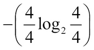
This is equal to 0.0.

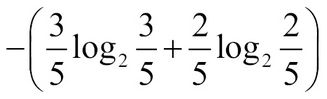
For sunny, out of 5 instances, only 2 have the value yes:

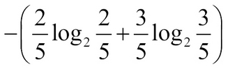
So the expected new entropy is given by the following formula:

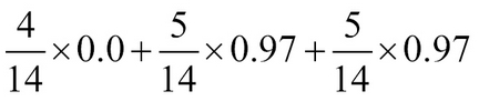
This is roughly equal to 0.69. If you follow these steps for the other attributes, you will find that the new entropies are like as follows:

So the highest information gain is attained if we split the dataset based on the outlook attribute.

Sometimes multiple trees are constructed by generating a random subset of all the available features. This technique is known as random forest.

Linear regression

Regression is used to predict the target value of the real valued variable. For example, let's say we have data about the number of bedrooms and the total area of many houses in a locality. We also have their prices listed as follows:

Number of Bedrooms	Total Area in square feet	Price
2	1150	2300000
3	2500	5600000
3	1780	4571030
4	3000	9000000

Now let's say we have this data in a real estate site's database and we want to create a feature to predict the price of a new house with three bedrooms and total area of 1650 square feet.

Linear regression is used to solve these types of problems. As you can see, these types of problems are pretty common.

In linear regression, you start with a model where you represent the target variable—the variable for which you want to predict the value. A polynomial model is selected that minimizes the least square error (this will be explained later in the chapter). Let me walk you through this example.

Each row of the available data can be represented as a tuple where the first few elements represent the value of the known/input parameters and the last parameter shows the value of the price (the target variable). So taking inspiration from mathematics, we can represent the unknown with and known as . Thus, each row can be represented as where to represent the parameters (the total area and the number of bedrooms) and represents the target value (the price of the house). Linear regression works on a model where y is represented with the x values.

The hypothesis is represented by an equation as the following. Here and theta denotes the input parameters (the number of bedrooms and the total area in square feet) and represents the predicted value of the new house.

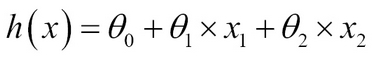
Note that this hypothesis is still a polynomial model and we are just using two features: the number of bedrooms and the total area represented by and .

So the square error is calculated by the following formula:

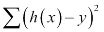
The task of linear regression is to choose a set of values for the coefficients which minimizes this error. The algorithm that minimizes this error is called gradient descent or batch gradient descent. You will learn more about it in Chapter 2, Linear Regression.

Logistic regression

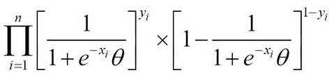
Unlike linear regression, logistic regression predicts a Boolean value indicating the class/tag/category of the target variable. Logistic regression is one of the most popular binary classifiers and is modelled by the equation that follows. and stands for the independent input variables and their classes/tags respectively. Logistic regression is discussed at length in Chapter 3, Classification Techniques.