
A simple linear regression has a single variable, and it can be described using the following formula:
y= A + Bx
Here, y is the dependent variable, x is the independent variable, A is the intercept (where x is to the power of zero) and B is the co-efficient
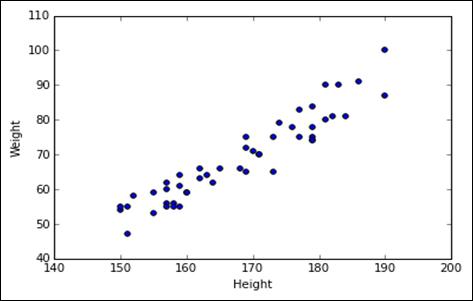
The dataset that we'll be using contains the height (cm) and weight (kg) of a sample of men.
The following code ingests the data and creates a simple scatter plot in order to understand the distribution of the weight versus the height:
>>> import numpy as np
>>> import pandas as pd
>>> from scipy import stats
>>> import matplotlib.pyplot as plt
>>> sl_data = pd.read_csv('Data/Mens_height_weight.csv')
>>> fig, ax = plt.subplots(1, 1)
>>> ax.scatter(sl_data['Height'],sl_data['Weight'])
>>> ax.set_xlabel('Height')
>>> ax.set_ylabel('Weight')
>>> plt.show()
The following is the output of the preceding code: