

There are many ways to define the DFT; however, in a NumPy implementation, the DFT is defined as the following equation:
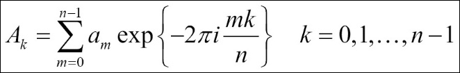
A k represents the discrete Fourier transform and am represents the original function. The transformation from am->Ak is a translation from the configuration space to the frequency space. Let's calculate this equation manually to get a better understanding of the transformation process. We will use a random signal with 500 values:
In [25]: x = np.random.random(500)
In [26]: n = len(x)
In [27]: m = np.arange(n)
In [28]: k = m.reshape((n, 1))
In [29]: M = np.exp(-2j * np.pi * k * m / n)
In [30]: y = np.dot(M, x)
In this code block, x is our simulated random signal, which contain 500 values and corresponds to am
in the equation. Based on the size of x, we calculate the sum product of:
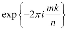
We then save it to M. The final step is to use the matrix multiplication between M and x to generate DFT and save it to y.
Let's...