Affinity analysis is a type of data mining that gives similarity between samples (objects). This could be the similarity between the following:

We can measure affinity in a number of ways. For instance, we can record how frequently two products are purchased together. We can also record the accuracy of the statement when a person buys object 1 and also when they buy object 2. Other ways to measure affinity include computing the similarity between samples, which we will cover in later chapters.

One of the issues with moving a traditional business online, such as commerce, is that tasks that used to be done by humans need to be automated in order for the online business to scale. One example of this is up-selling, or selling an extra item to a customer who is already buying. Automated product recommendations through data mining are one of the driving forces behind the e-commerce revolution that is turning billions of dollars per year into revenue.

In this example, we are going to focus on a basic product recommendation service. We design this based on the following idea: when two items are historically purchased together, they are more likely to be purchased together in the future. This sort of thinking is behind many product recommendation services, in both online and offline businesses.

A very simple algorithm for this type of product recommendation algorithm is to simply find any historical case where a user has brought an item and to recommend other items that the historical user brought. In practice, simple algorithms such as this can do well, at least better than choosing random items to recommend. However, they can be improved upon significantly, which is where data mining comes in.

To simplify the coding, we will consider only two items at a time. As an example, people may buy bread and milk at the same time at the supermarket. In this early example, we wish to find simple rules of the form:

If a person buys product X, then they are likely to purchase product Y

More complex rules involving multiple items will not be covered such as people buying sausages and burgers being more likely to buy tomato sauce.

The dataset can be downloaded from the code package supplied with the book. Download this file and save it on your computer, noting the path to the dataset. For this example, I recommend that you create a new folder on your computer to put your dataset and code in. From here, open your IPython Notebook, navigate to this folder, and create a new notebook.

The dataset we are going to use for this example is a NumPy two-dimensional array, which is a format that underlies most of the examples in the rest of the book. The array looks like a table, with rows representing different samples and columns representing different features.

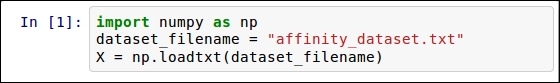
The cells represent the value of a particular feature of a particular sample. To illustrate, we can load the dataset with the following code:

import numpy as np
dataset_filename = "affinity_dataset.txt"
X = np.loadtxt(dataset_filename)

For this example, run the IPython Notebook and create an IPython Notebook. Enter the above code into the first cell of your Notebook. You can then run the code by pressing Shift + Enter (which will also add a new cell for the next lot of code). After the code is run, the square brackets to the left-hand side of the first cell will be assigned an incrementing number, letting you know that this cell has been completed. The first cell should look like the following:

For later code that will take more time to run, an asterisk will be placed here to denote that this code is either running or scheduled to be run. This asterisk will be replaced by a number when the code has completed running.

You will need to save the dataset into the same directory as the IPython Notebook. If you choose to store it somewhere else, you will need to change the dataset_filename value to the new location.

Next, we can show some of the rows of the dataset to get a sense of what the dataset looks like. Enter the following line of code into the next cell and run it, in order to print the first five lines of the dataset:

print(X[:5])

The result will show you which items were bought in the first five transactions listed:

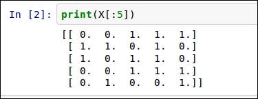
The dataset can be read by looking at each row (horizontal line) at a time. The first row (0, 0, 1, 1, 1) shows the items purchased in the first transaction. Each column (vertical row) represents each of the items. They are bread, milk, cheese, apples, and bananas, respectively. Therefore, in the first transaction, the person bought cheese, apples, and bananas, but not bread or milk.

Each of these features contain binary values, stating only whether the items were purchased and not how many of them were purchased. A 1 indicates that "at least 1" item was bought of this type, while a 0 indicates that absolutely none of that item was purchased.

We wish to find rules of the type If a person buys product X, then they are likely to purchase product Y. We can quite easily create a list of all of the rules in our dataset by simply finding all occasions when two products were purchased together. However, we then need a way to determine good rules from bad ones. This will allow us to choose specific products to recommend.

Rules of this type can be measured in many ways, of which we will focus on two: support and confidence.

Support is the number of times that a rule occurs in a dataset, which is computed by simply counting the number of samples that the rule is valid for. It can sometimes be normalized by dividing by the total number of times the premise of the rule is valid, but we will simply count the total for this implementation.

While the support measures how often a rule exists, confidence measures how accurate they are when they can be used. It can be computed by determining the percentage of times the rule applies when the premise applies. We first count how many times a rule applies in our dataset and divide it by the number of samples where the premise (the if statement) occurs.

As an example, we will compute the support and confidence for the rule if a person buys apples, they also buy bananas.

As the following example shows, we can tell whether someone bought apples in a transaction by checking the value of sample[3], where a sample is assigned to a row of our matrix:

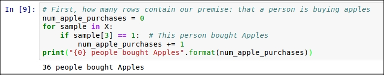
Similarly, we can check if bananas were bought in a transaction by seeing if the value for sample[4] is equal to 1 (and so on). We can now compute the number of times our rule exists in our dataset and, from that, the confidence and support.

Now we need to compute these statistics for all rules in our database. We will do this by creating a dictionary for both valid rules and invalid rules. The key to this dictionary will be a tuple (premise and conclusion). We will store the indices, rather than the actual feature names. Therefore, we would store (3 and 4) to signify the previous rule If a person buys Apples, they will also buy Bananas. If the premise and conclusion are given, the rule is considered valid. While if the premise is given but the conclusion is not, the rule is considered invalid for that sample.

To compute the confidence and support for all possible rules, we first set up some dictionaries to store the results. We will use defaultdict for this, which sets a default value if a key is accessed that doesn't yet exist. We record the number of valid rules, invalid rules, and occurrences of each premise:

from collections import defaultdict
valid_rules = defaultdict(int)
invalid_rules = defaultdict(int)
num_occurances = defaultdict(int)

Next we compute these values in a large loop. We iterate over each sample and feature in our dataset. This first feature forms the premise of the rule—if a person buys a product premise:

for sample in X:
  for premise in range(4):

We check whether the premise exists for this sample. If not, we do not have any more processing to do on this sample/premise combination, and move to the next iteration of the loop:

  if sample[premise] == 0: continue

If the premise is valid for this sample (it has a value of 1), then we record this and check each conclusion of our rule. We skip over any conclusion that is the same as the premise—this would give us rules such as If a person buys Apples, then they buy Apples, which obviously doesn't help us much;

  num_occurances[premise] += 1
  for conclusion in range(n_features):
      if premise == conclusion: continue

If the conclusion exists for this sample, we increment our valid count for this rule. If not, we increment our invalid count for this rule:

  if sample[conclusion] == 1:
    valid_rules[(premise, conclusion)] += 1
    else:
    invalid_rules[(premise, conclusion)] += 1

We have now completed computing the necessary statistics and can now compute the support and confidence for each rule. As before, the support is simply our valid_rules value:

support = valid_rules

The confidence is computed in the same way, but we must loop over each rule to compute this:

confidence = defaultdict(float)
for premise, conclusion in valid_rules.keys():
    rule = (premise, conclusion)
    confidence[rule] = valid_rules[rule] / num_occurances[premise]

We now have a dictionary with the support and confidence for each rule. We can create a function that will print out the rules in a readable format. The signature of the rule takes the premise and conclusion indices, the support and confidence dictionaries we just computed, and the features array that tells us what the features mean:

def print_rule(premise, conclusion,
              support, confidence, features):

We get the names of the features for the premise and conclusion and print out the rule in a readable format:

    premise_name = features[premise]
    conclusion_name = features[conclusion]
    print("Rule: If a person buys {0} they will also buy 
      {1}".format(premise_name, conclusion_name))

Then we print out the Support and Confidence of this rule:

    print(" - Support: {0}".format(support[(premise,
                                            conclusion)]))
    print(" - Confidence: {0:.3f}".format(confidence[(premise,
                                                    conclusion)]))

We can test the code by calling it in the following way—feel free to experiment with different premises and conclusions:

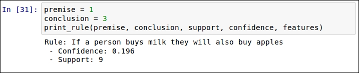
Now that we can compute the support and confidence of all rules, we want to be able to find the best rules. To do this, we perform a ranking and print the ones with the highest values. We can do this for both the support and confidence values.

To find the rules with the highest support, we first sort the support dictionary. Dictionaries do not support ordering by default; the items() function gives us a list containing the data in the dictionary. We can sort this list using the itemgetter class as our key, which allows for the sorting of nested lists such as this one. Using itemgetter(1) allows us to sort based on the values. Setting reverse=True gives us the highest values first:

from operator import itemgetter
 sorted_support = sorted(support.items(), key=itemgetter(1), reverse=True)

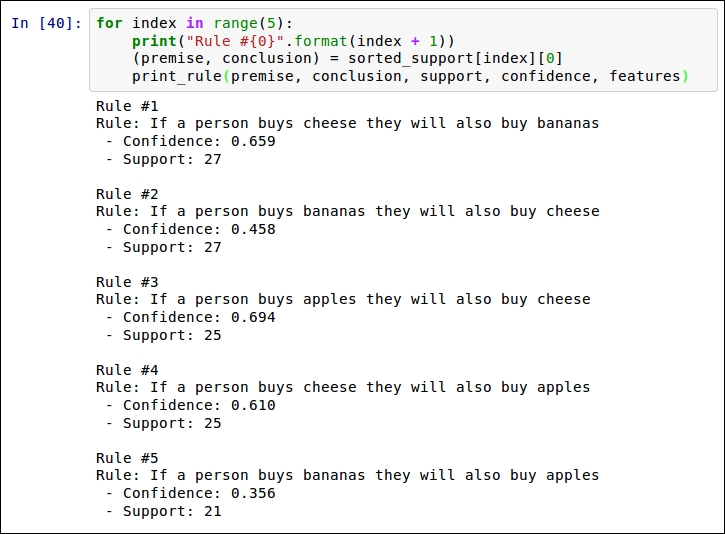
We can then print out the top five rules:

for index in range(5):
    print("Rule #{0}".format(index + 1))
    premise, conclusion = sorted_support[index][0]
    print_rule(premise, conclusion, support, confidence, features)

The result will look like the following:

Similarly, we can print the top rules based on confidence. First, compute the sorted confidence list:

sorted_confidence = sorted(confidence.items(), key=itemgetter(1), reverse=True)

Next, print them out using the same method as before. Note the change to sorted_confidence on the third line;

for index in range(5):
    print("Rule #{0}".format(index + 1))
    premise, conclusion = sorted_confidence[index][0]
    print_rule(premise, conclusion, support, confidence, features)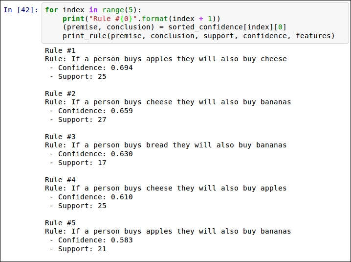

Two rules are near the top of both lists. The first is If a person buys apples, they will also buy cheese, and the second is If a person buys cheese, they will also buy bananas. A store manager can use rules like these to organize their store. For example, if apples are on sale this week, put a display of cheeses nearby. Similarly, it would make little sense to put both bananas on sale at the same time as cheese, as nearly 66 percent of people buying cheese will buy bananas anyway—our sale won't increase banana purchases all that much.

Data mining has great exploratory power in examples like this. A person can use data mining techniques to explore relationships within their datasets to find new insights. In the next section, we will use data mining for a different purpose: prediction.