R provides a complete series of options to realize graphics, which makes it quite advanced with regard to data visualization. Along the next few sections of this chapter, we will go through the most important R packages for data visualization by quickly discussing some high-level differences and analogies. If you already have some experience with other R packages for data visualization, in particular graphics or lattice, the following sections will provide you with some references and examples of how the code used in such packages appears in comparison with that used in ggplot2. Moreover, you will also have an idea of the typical layout of the plots created with a certain package, so you will be able to identify the tool used to realize the plots you will come across.

The core of graphics visualization in R is within the grDevices package, which provides the basic structure of data plotting, such as the colors and fonts used in the plots. Such a graphic engine was then used as the starting point in the development of more advanced and sophisticated packages for data visualization, the most commonly used being graphics and grid.

The graphics package is often referred to as the base or traditional graphics environment since, historically, it was the first package for data visualization available in R, and it provides functions that allow the generation of complete plots.

The grid package, on the other hand, provides an alternative set of graphics tools. This package does not directly provide functions that generate complete plots, so it is not frequently used directly to generate graphics, but it is used in the development of advanced data visualization packages. Among the grid-based packages, the most widely used are lattice and ggplot2, although they are built by implementing different visualization approaches—Trellis plots in the case of lattice and the grammar of graphics in the case of ggplot2. We will describe these principles in more detail in the coming sections. A diagram representing the connections between the tools just mentioned is shown in Figure 1.2. Just keep in mind that this is not a complete overview of the packages available but simply a small snapshot of the packages we will discuss. Many other packages are built on top of the tools just mentioned, but in the following sections, we will focus on the most relevant packages used in data visualization, namely graphics, lattice, and, of course, ggplot2. If you would like to get a more complete overview of the graphics tools available in R, you can have a look at the web page of the R project summarizing such tools, http://cran.r-project.org/web/views/Graphics.html.

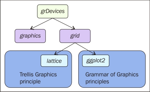
Figure 1.2: This is an overview of the most widely used R packages for graphics

In order to see some examples of plots in graphics, lattice and ggplot2, we will go through a few examples of different plots over the following pages. The objective of providing these examples is not to do an exhaustive comparison of the three packages but simply to provide you with a simple comparison of how the different codes as well as the default plot layouts appear for these different plotting tools. For these examples, we will use the Orange dataset available in R; to load it in the workspace, simply write the following code:

>data(Orange)

This dataset contains records of the growth of orange trees. You can have a look at the data by recalling its first lines with the following code:

>head(Orange)

You will see that the dataset contains three columns. The first one, Tree, is an ID number indicating the tree on which the measurement was taken, while age and circumference refer to the age in days and the size of the tree in millimeters, respectively. If you want to have more information about this data, you can have a look at the help page of the dataset by typing the following code:

?Orange

Here, you will find the reference of the data as well as a more detailed description of the variables included.