
In this recipe we will examine how regression can be viewed as being very similar to classification. This is done by reconsidering the categorical labels of regression as real numbers. In this section we will also look at at several aspects of machine learning from a very broad perspective including the purpose of scikit-learn. scikit-learn allows us to find models that work well incredibly quickly. We do not have to work out all the details of the model, or optimize, until we found one that works well. Consequently, your company saves precious development time and computational resources thanks to scikit-learn giving us the ability to develop models relatively quickly.
Machine learning overview – classification versus regression
The purpose of scikit-learn
As we have seen before, scikit-learn allowed us to find a model that works fairly quickly. We tried SVC, logistic regression, and a few KNN classifiers. Through cross-validation, we selected models that performed better than others. In industry, after trying SVMs and logistic regression, we might focus on SVMs and optimize them further. Thanks to scikit-learn, we saved a lot of time and resources, including mental energy. After optimizing the SVM at work on a realistic dataset, we might re-implement it for speed in Java or C and gather more data.
Supervised versus unsupervised
Classification and regression are supervised, as we know the target variables for the observations. Clustering—creating regions in space for each category without being given any labels is unsupervised learning.
Getting ready
In classification, the target variable is one of several categories, and there must be more than one instance of every category. In regression, there can be only one instance of every target variable, as the only requirement is that the target is a real number.
In the case of logistic regression, we saw previously that the algorithm first performs a regression and estimates a real number for the target. Then the target class is estimated by using thresholds. In scikit-learn, there are predict_proba methods that yield probabilistic estimates, which relate regression-like real number estimates with classification classes in the style of logistic regression.
Any regression can be turned into classification by using thresholds. A binary classification can be viewed as a regression problem by using a regressor. The target variables produced will be real numbers, not the original class variables.
How to do it...
Quick SVC – a classifier and regressor
- Load iris from the datasets module:
import numpy as np
import pandas as pd
from sklearn import datasets

iris = datasets.load_iris()
- For simplicity, consider only targets 0 and 1, corresponding to Setosa and Versicolor. Use the Boolean array iris.target < 2 to filter out target 2. Place it within brackets to use it as a filter in defining the observation set X and the target set y:
X = iris.data[iris.target < 2]
y = iris.target[iris.target < 2]
- Now import train_test_split and apply it:
from sklearn.model_selection import train_test_split
from sklearn.metrics import accuracy_score

X_train, X_test, y_train, y_test = train_test_split(X, y, stratify=y, random_state= 7)
- Prepare and run an SVC by importing it and scoring it with cross-validation:
from sklearn.svm import SVC
from sklearn.model_selection import cross_val_score

svc_clf = SVC(kernel = 'linear').fit(X_train, y_train)
svc_scores = cross_val_score(svc_clf, X_train, y_train, cv=4)
- As done in previous sections, view the average of the scores:
svc_scores.mean()

0.94795321637426899
- Perform the same with support vector regression by importing SVR from sklearn.svm, the same module that contains SVC:
from sklearn.svm import SVR
- Then write the necessary syntax to fit the model. It is almost identical to the syntax for SVC, just replacing some c keywords with r:
svr_clf = SVR(kernel = 'linear').fit(X_train, y_train)
Making a scorer
To make a scorer, you need:
- A scoring function that compares y_test, the ground truth, with y_pred, the predictions
- To determine whether a high score is good or bad
Before passing the SVR regressor to the cross-validation, make a scorer by supplying two elements:
- In practice, begin by importing the make_scorer function:
from sklearn.metrics import make_scorer
- Use this sample scoring function:
#Only works for this iris example with targets 0 and 1
def for_scorer(y_test, orig_y_pred):
    y_pred = np.rint(orig_y_pred).astype(np.int)   #rounds prediction to the nearest integer
    return accuracy_score(y_test, y_pred)
The np.rint function rounds off the prediction to the nearest integer, hopefully one of the targets, 0 or 1. The astype method changes the type of the prediction to integer type, as the original target is in integer type and consistency is preferred with regard to types. After the rounding occurs, the scoring function uses the old accuracy_score function, which you are familiar with.
- Now, determine whether a higher score is better. Higher accuracy is better, so for this situation, a higher score is better. In scikit code:
svr_to_class_scorer = make_scorer(for_scorer, greater_is_better=True)
- Finally, run the cross-validation with a new parameter, the scoring parameter:
svr_scores = cross_val_score(svr_clf, X_train, y_train, cv=4, scoring = svr_to_class_scorer)
- Find the mean:
svr_scores.mean()

0.94663742690058483
The accuracy scores are similar for the SVR regressor-based classifier and the traditional SVC classifier.
How it works...
You might ask, why did we take out class 2 out of the target set?
The reason is that, to use a regressor, our intent has to be to predict a real number. The categories had to have real number properties: that they are ordered (informally, if we have three ordered categories x, y, z and x < y and y < z then x < z). By eliminating the third category, the remaining flowers (Setosa and Versicolor) became ordered by a property we invented: Setosaness or Versicolorness.
The next time you encounter categories, you can consider whether they can be ordered. For example, if the dataset consists of shoe sizes, they can be ordered and a regressor can be applied, even though no one has a shoe size of 12.125.
There's more...
Linear versus nonlinear
Linear algorithms involve lines or hyperplanes. Hyperplanes are flat surfaces in any n-dimensional space. They tend to be easy to understand and explain, as they involve ratios (with an offset). Some functions that consistently and monotonically increase or decrease can be mapped to a linear function with a transformation. For example, exponential growth can be mapped to a line with the log transformation.
Nonlinear algorithms tend to be tougher to explain to colleagues and investors, yet ensembles of decision trees that are nonlinear tend to perform very well. KNN, which we examined earlier, is nonlinear. In some cases, functions not increasing or decreasing in a familiar manner are acceptable for the sake of accuracy.
Try a simple SVC with a polynomial kernel, as follows:
from sklearn.svm import SVC   #Usual import of SVC
svc_poly_clf = SVC(kernel = 'poly', degree= 3).fit(X_train, y_train)  #Polynomial Kernel of Degree 3
The polynomial kernel of degree 3 looks like a cubic curve in two dimensions. It leads to a slightly better fit, but note that it can be harder to explain to others than a linear kernel with consistent behavior throughout all of the Euclidean space:
svc_poly_scores = cross_val_score(svc_clf, X_train, y_train, cv=4)
svc_poly_scores.mean()

0.95906432748538006
Black box versus not
For the sake of efficiency, we did not examine the classification algorithms used very closely. When we compared SVC and logistic regression, we chose SVMs. At that point, both algorithms were black boxes, as we did not know any internal details. Once we decided to focus on SVMs, we could proceed to compute coefficients of the separating hyperplanes involved, optimize the hyperparameters of the SVM, use the SVM for big data, and do other processes. The SVMs have earned our time investment because of their superior performance.
Interpretability
Some machine learning algorithms are easier to understand than others. These are usually easier to explain to others as well. For example, linear regression is well known and easy to understand and explain to potential investors of your company. SVMs are more difficult to entirely understand.
My general advice: if SVMs are highly effective for a particular dataset, try to increase your personal interpretability of SVMs in the particular problem context. Also, consider merging algorithms somehow, using linear regression as an input to SVMs, for example. This way, you have the best of both worlds.
This is really context-specific, however. Linear SVMs are relatively simple to visualize and understand. Merging linear regression with SVM could complicate things. You can start by comparing them side by side.
However, if you cannot understand every detail of the math and practice of SVMs, be kind to yourself, as machine learning is focused more on prediction performance rather than traditional statistics.
A pipeline
In programming, a pipeline is a set of procedures connected in series, one after the other, where the output of one process is the input to the next:
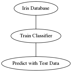
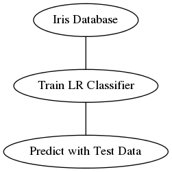
You can replace any procedure in the process with a different one, perhaps better in some way, without compromising the whole system. For the model in the middle step, you can use an SVC or logistic regression:
One can also keep track of the classifier itself and build a flow diagram from the classifier. Here is a pipeline keeping track of the SVC classifier:
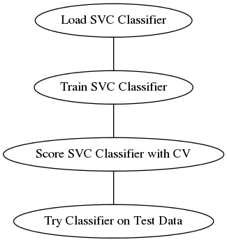
In the upcoming chapters, we will see how scikit-learn uses the intuitive notion of a pipeline. So far, we have used a simple one: train, predict, test.