A data flow graph or computation graph is the basic unit of computation in TensorFlow. We will refer to them as the computation graph from now on. A computation graph is made up of nodes and edges. Each node represents an operation (tf.Operation) and each edge represents a tensor (tf.Tensor) that gets transferred between the nodes.

A program in TensorFlow is basically a computation graph. You create the graph with nodes representing variables, constants, placeholders, and operations and feed it to TensorFlow. TensorFlow finds the first nodes that it can fire or execute. The firing of these nodes results in the firing of other nodes, and so on.

Thus, TensorFlow programs are made up of two kinds of operations on computation graphs:

• Building the computation graph
• Running the computation graph

The TensorFlow comes with a default graph. Unless another graph is explicitly specified, a new node gets implicitly added to the default graph. We can get explicit access to the default graph using the following command:

graph = tf.get_default_graph()

For example, if we want to define three inputs and add them to produce output , we can represent it using the following computation graph:

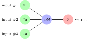
In TensorFlow, the add operation in the preceding image would correspond to the code y = tf.add( x1 + x2 + x3 ).

As we create the variables, constants, and placeholders, they get added to the graph. Then we create a session object to execute the operation objects and evaluate the tensor objects.

Let's build and execute a computation graph to calculate , as we already saw in the preceding example:

# Assume Linear Model y = w * x + b
# Define model parameters
w = tf.Variable([.3], tf.float32)
b = tf.Variable([-.3], tf.float32)
# Define model input and output
x = tf.placeholder(tf.float32)
y = w * x + b
output = 0

with tf.Session() as tfs:
   # initialize and print the variable y
   tf.global_variables_initializer().run()
   output = tfs.run(y,{x:[1,2,3,4]})
print('output : ',output)

Creating and using a session in the with block ensures that the session is automatically closed when the block is finished. Otherwise, the session has to be explicitly closed with the tfs.close() command, where tfs is the session name.

The nodes are executed in the order of dependency. If node a depends on node b, then a will be executed before b when the execution of b is requested. A node is not executed unless either the node itself or another node depending on it is not requested for execution. This is also known as lazy loading; namely, the node objects are not created and initialized until they are needed.

Sometimes, you may want to control the order in which the nodes are executed in a graph. This can be achieved with the tf.Graph.control_dependencies() function. For example, if the graph has nodes a, b, c, and d and you want to execute c and d before a and b, then use the following statement:

with graph_variable.control_dependencies([c,d]):
  # other statements here

This makes sure that any node in the preceding with block is executed only after nodes c and d have been executed.

A graph can be divided into multiple parts and each part can be placed and executed on separate devices, such as a CPU or GPU. You can list all the devices available for graph execution with the following command:

from tensorflow.python.client import device_lib
print(device_lib.list_local_devices())

We get the following output (your output would be different, depending on the compute devices in your system):

[name: "/device:CPU:0"
device_type: "CPU"
memory_limit: 268435456
locality {
}
incarnation: 12900903776306102093
, name: "/device:GPU:0"
device_type: "GPU"
memory_limit: 611319808
locality {
  bus_id: 1
}
incarnation: 2202031001192109390
physical_device_desc: "device: 0, name: Quadro P5000, pci bus id: 0000:01:00.0, compute capability: 6.1"
]

The devices in TensorFlow are identified with the string /device:<device_type>:<device_idx>. In the above output, the CPU and GPU denote the device type and 0 denotes the device index.

One thing to note about the above output is that it shows only one CPU, whereas our computer has 8 CPUs. The reason for that is TensorFlow implicitly distributes the code across the CPU units and thus by default CPU:0 denotes all the CPU's available to TensorFlow. When TensorFlow starts executing graphs, it runs the independent paths within each graph in a separate thread, with each thread running on a separate CPU. We can restrict the number of threads used for this purpose by changing the number of inter_op_parallelism_threads. Similarly, if within an independent path, an operation is capable of running on multiple threads, TensorFlow will launch that specific operation on multiple threads. The number of threads in this pool can be changed by setting the number of intra_op_parallelism_threads.

Let us enable the logging of variable placement by defining a config object, set the log_device_placement property to true, and then pass this config object to the session as follows:

tf.reset_default_graph()

# Define model parameters
w = tf.Variable([.3], tf.float32)
b = tf.Variable([-.3], tf.float32)
# Define model input and output
x = tf.placeholder(tf.float32)
y = w * x + b

config = tf.ConfigProto()
config.log_device_placement=True

with tf.Session(config=config) as tfs:
   # initialize and print the variable y
   tfs.run(global_variables_initializer())
   print('output',tfs.run(y,{x:[1,2,3,4]}))

We get the following output in Jupyter Notebook console:

b: (VariableV2): /job:localhost/replica:0/task:0/device:GPU:0
b/read: (Identity): /job:localhost/replica:0/task:0/device:GPU:0
b/Assign: (Assign): /job:localhost/replica:0/task:0/device:GPU:0
w: (VariableV2): /job:localhost/replica:0/task:0/device:GPU:0
w/read: (Identity): /job:localhost/replica:0/task:0/device:GPU:0
mul: (Mul): /job:localhost/replica:0/task:0/device:GPU:0
add: (Add): /job:localhost/replica:0/task:0/device:GPU:0
w/Assign: (Assign): /job:localhost/replica:0/task:0/device:GPU:0
init: (NoOp): /job:localhost/replica:0/task:0/device:GPU:0
x: (Placeholder): /job:localhost/replica:0/task:0/device:GPU:0
b/initial_value: (Const): /job:localhost/replica:0/task:0/device:GPU:0
Const_1: (Const): /job:localhost/replica:0/task:0/device:GPU:0
w/initial_value: (Const): /job:localhost/replica:0/task:0/device:GPU:0
Const: (Const): /job:localhost/replica:0/task:0/device:GPU:0

Thus by default, the TensorFlow creates the variable and operations nodes on a device where it can get the highest performance. The variables and operations can be placed on specific devices by using tf.device() function. Let us place the graph on the CPU:

tf.reset_default_graph()

with tf.device('/device:CPU:0'):
    # Define model parameters
    w = tf.get_variable(name='w',initializer=[.3], dtype=tf.float32)
    b = tf.get_variable(name='b',initializer=[-.3], dtype=tf.float32)
    # Define model input and output
    x = tf.placeholder(name='x',dtype=tf.float32)
    y = w * x + b

config = tf.ConfigProto()
config.log_device_placement=True

with tf.Session(config=config) as tfs:
   # initialize and print the variable y
   tfs.run(tf.global_variables_initializer())
   print('output',tfs.run(y,{x:[1,2,3,4]}))

In the Jupyter console we see that now the variables have been placed on the CPU and the execution also takes place on the CPU:

b: (VariableV2): /job:localhost/replica:0/task:0/device:CPU:0
b/read: (Identity): /job:localhost/replica:0/task:0/device:CPU:0
b/Assign: (Assign): /job:localhost/replica:0/task:0/device:CPU:0
w: (VariableV2): /job:localhost/replica:0/task:0/device:CPU:0
w/read: (Identity): /job:localhost/replica:0/task:0/device:CPU:0
mul: (Mul): /job:localhost/replica:0/task:0/device:CPU:0
add: (Add): /job:localhost/replica:0/task:0/device:CPU:0
w/Assign: (Assign): /job:localhost/replica:0/task:0/device:CPU:0
init: (NoOp): /job:localhost/replica:0/task:0/device:CPU:0
x: (Placeholder): /job:localhost/replica:0/task:0/device:CPU:0
b/initial_value: (Const): /job:localhost/replica:0/task:0/device:CPU:0
Const_1: (Const): /job:localhost/replica:0/task:0/device:CPU:0
w/initial_value: (Const): /job:localhost/replica:0/task:0/device:CPU:0
Const: (Const): /job:localhost/replica:0/task:0/device:CPU:0

TensorFlow follows these simple rules, also known as the simple placement, for placing the variables on the devices:

If the graph was previously run, 
    then the node is left on the device where it was placed earlier
Else If the tf.device() block is used,
    then the node is placed on the specified device
Else If the GPU is present
    then the node is placed on the first available GPU
Else If the GPU is not present
    then the node is placed on the CPU

The tf.device() can also be passed a function name instead of a device string. In such case, the function must return the device string. This feature allows complex algorithms for placing the variables on different devices. For example, TensorFlow provides a round robin device setter in tf.train.replica_device_setter() that we will discuss later in next section.

When you place a TensorFlow operation on the GPU, the TF must have the GPU implementation of that operation, known as the kernel. If the kernel is not present then the placement results in run-time error. Also if the GPU device you requested does not exist, you will get a run-time error. The best way to handle such errors is to allow the operation to be placed on the CPU if requesting the GPU device results in n error. This can be achieved by setting the following config value:

config.allow_soft_placement = True

When you start running the TensorFlow session, by default it grabs all of the GPU memory, even if you place the operations and variables only on one GPU in a multi-GPU system. If you try to run another session at the same time, you will get out of memory error. This can be solved in multiple ways:

• For multi-GPU systems, set the environment variable CUDA_VISIBLE_DEVICES=<list of device idx>

os.environ['CUDA_VISIBLE_DEVICES']='0'

The code executed after this setting will be able to grab all of the memory of only the visible GPU.

• When you do not want the session to grab all of the memory of the GPU, then you can use the config option per_process_gpu_memory_fraction to allocate a percentage of memory:

config.gpu_options.per_process_gpu_memory_fraction = 0.5

This will allocate 50% of the memory of all the GPU devices.

• You can also combine both of the above strategies, i.e. make only a percentage along with making only some of the GPU visible to the process.
• You can also limit the TensorFlow process to grab only the minimum required memory at the start of the process. As the process executes further, you can set a config option to allow the growth of this memory.

config.gpu_options.allow_growth = True

This option only allows for the allocated memory to grow, but the memory is never released back.

You will learn techniques for distributing computation across multiple compute devices and multiple nodes in later chapters.

You can create your own graphs separate from the default graph and execute them in a session. However, creating and executing multiple graphs is not recommended, as it has the following disadvantages:

• Creating and using multiple graphs in the same program would require multiple TensorFlow sessions and each session would consume heavy resources
• You cannot directly pass data in between graphs

Hence, the recommended approach is to have multiple subgraphs in a single graph. In case you wish to use your own graph instead of the default graph, you can do so with the tf.graph() command. Here is an example where we create our own graph, g, and execute it as the default graph:

g = tf.Graph()
output = 0

# Assume Linear Model y = w * x + b

with g.as_default():
 # Define model parameters
 w = tf.Variable([.3], tf.float32)
 b = tf.Variable([-.3], tf.float32)
 # Define model input and output
 x = tf.placeholder(tf.float32)
 y = w * x + b

with tf.Session(graph=g) as tfs:
 # initialize and print the variable y
 tf.global_variables_initializer().run()
 output = tfs.run(y,{x:[1,2,3,4]})
 
print('output : ',output)