
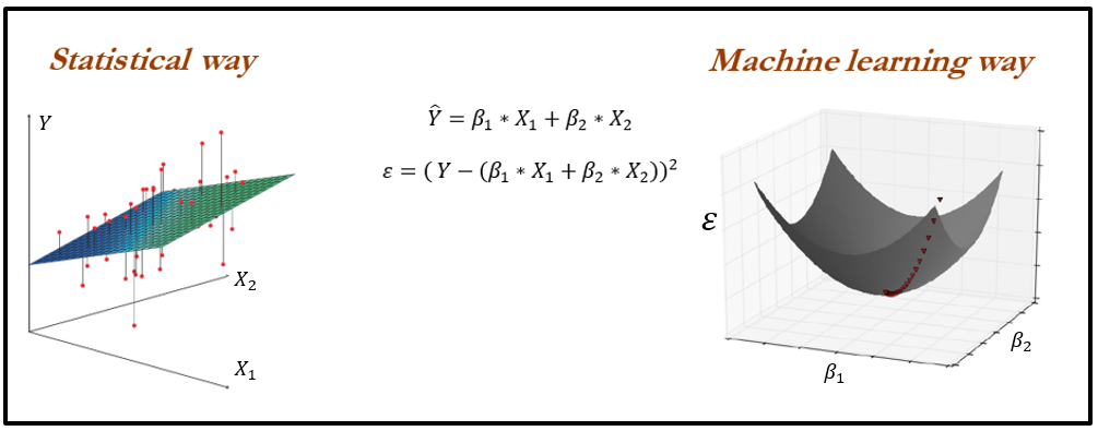
There seems to be an analogy between statistical modeling and machine learning that we will cover in subsequent chapters in depth. However, a quick view has been provided as follows: in statistical modeling, linear regression with two independent variables is trying to fit the best plane with the least errors, whereas in machine learning independent variables have been converted into the square of error terms (squaring ensures the function will become convex, which enhances faster convergence and also ensures a global optimum) and optimized based on coefficient values rather than independent variables:
Machine learning utilizes optimization for tuning all the parameters of various algorithms. Hence, it is a good idea to know some basics about optimization.
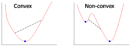
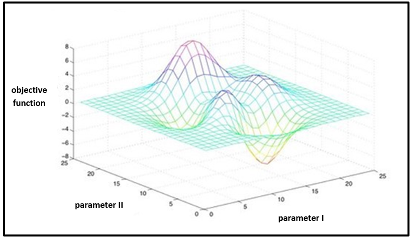
Before stepping into gradient descent, the introduction of convex and non-convex functions is very helpful. Convex functions are functions in which a line drawn between any two random points on the function also lies within the function, whereas this isn't true for non-convex functions. It is important to know whether the function is convex or non-convex due to the fact that in convex functions, the local optimum is also the global optimum, whereas for non-convex functions, the local optimum does not guarantee the global optimum:
Does it seem like a tough problem? One turnaround could be to initiate a search process at different random locations; by doing so, it usually converges to the global optimum:
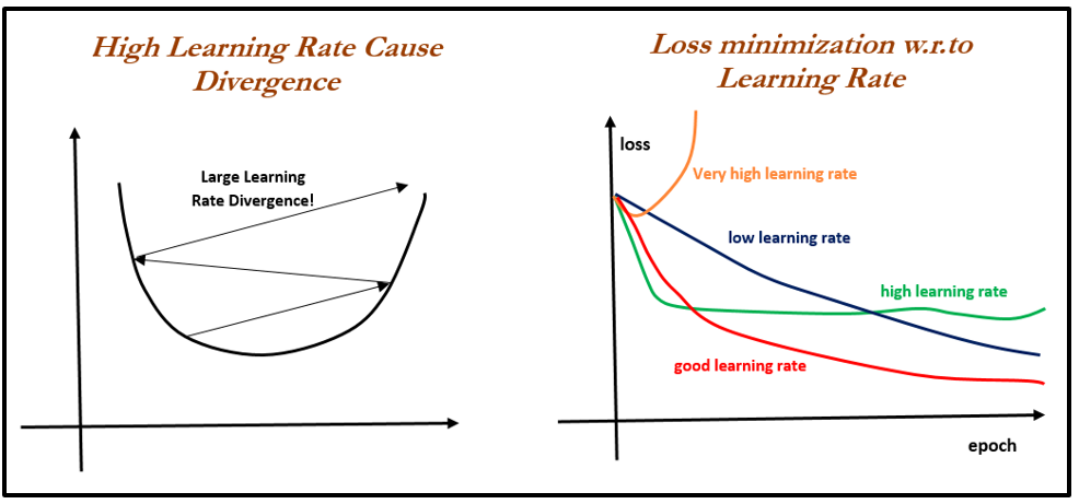
- Gradient descent: This is a way to minimize the objective function J(Θ) parameterized by the model's parameter Θε Rd by updating the parameters in the opposite direction to the gradient of the objective function with respect to the parameters. The learning rate determines the size of steps taken to reach the minimum.
- Full batch gradient descent (all training observations considered in each and every iteration): In full batch gradient descent, all the observations are considered for each and every iteration; this methodology takes a lot of memory and will be slow as well. Also, in practice, we do not need to have all the observations to update the weights. Nonetheless, this method provides the best way of updating parameters with less noise at the expense of huge computation.
- Stochastic gradient descent (one observation per iteration): This method updates weights by taking one observation at each stage of iteration. This method provides the quickest way of traversing weights; however, a lot of noise is involved while converging.
- Mini batch gradient descent (about 30 training observations or more for each and every iteration): This is a trade-off between huge computational costs and a quick method of updating weights. In this method, at each iteration, about 30 observations will be selected at random and gradients calculated to update the model weights. Here, a question many can ask is, why the minimum 30 and not any other number? If we look into statistical basics, 30 observations required to be considering in order approximating sample as a population. However, even 40, 50, and so on will also do well in batch size selection. Nonetheless, a practitioner needs to change the batch size and verify the results, to determine at what value the model is producing the optimum results:
In the following code, a comparison has been made between applying linear regression in a statistical way and gradient descent in a machine learning way on the same dataset:
>>> import numpy as np
>>> import pandas as pd
The following code describes reading data using a pandas DataFrame:
>>> train_data = pd.read_csv("mtcars.csv") Converting DataFrame variables into NumPy arrays in order to process them in scikit learn packages, as scikit-learn is built on NumPy arrays itself, is shown next:
>>> X = np.array(train_data["hp"])  ; y = np.array(train_data["mpg"])
>>> X = X.reshape(32,1); y = y.reshape(32,1)
Importing linear regression from the scikit-learn package; this works on the least squares method:
>>> from sklearn.linear_model import LinearRegression
>>> model = LinearRegression(fit_intercept = True)
Fitting a linear regression model on the data and display intercept and coefficient of single variable (hp variable):
>>> model.fit(X,y)
>>> print ("Linear Regression Results" )
>>> print ("Intercept",model.intercept_[0] ,"Coefficient", model.coef_[0])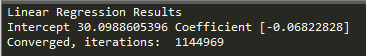
Now we will apply gradient descent from scratch; in future chapters, we can use the scikit-learn built-in modules rather than doing it from first principles. However, here, an illustration has been provided on the internal workings of the optimization method on which the whole machine learning has been built.
Defining the gradient descent function gradient_descent with the following:
x: Independent variable.y: Dependent variable.learn_rate: Learning rate with which gradients are updated; too low causes slower convergence and too high causes overshooting of gradients.batch_size: Number of observations considered at each iteration for updating gradients; a high number causes a lower number of iterations and a lower number causes an erratic decrease in errors. Ideally, the batch size should be a minimum value of 30 due to statistical significance. However, various settings need to be tried to check which one is better.max_iter: Maximum number of iteration, beyond which the algorithm will get auto-terminated:
>>> def gradient_descent(x, y,learn_rate, conv_threshold,batch_size, max_iter):
...    converged = False
...    iter = 0
...    m = batch_size
...    t0 = np.random.random(x.shape[1])
...    t1 = np.random.random(x.shape[1])
Note
Mean square error calculationSquaring of error has been performed to create the convex function, which has nice convergence properties:... MSE = (sum([(t0 + t1*x[i] - y[i])**2 for i in range(m)])/ m)
The following code states, run the algorithm until it does not meet the convergence criteria:
...      while not converged:
...          grad0 = 1.0/m * sum([(t0 + t1*x[i] - y[i]) for i in range(m)])
...          grad1 = 1.0/m * sum([(t0 + t1*x[i] - y[i])*x[i] for i in range(m)])
...          temp0 = t0 - learn_rate * grad0
...          temp1 = t1 - learn_rate * grad1
...          t0 = temp0
...          t1 = temp1
Calculate a new error with updated parameters, in order to check whether the new error changed more than the predefined convergence threshold value; otherwise, stop the iterations and return parameters:
...          MSE_New = (sum( [ (t0 + t1*x[i] - y[i])**2 for i in range(m)] ) / m)
...          if abs(MSE - MSE_New ) <= conv_threshold:
...              print 'Converged, iterations: ', iter
...              converged = True
...          MSE = MSE_New
...          iter += 1
...          if iter == max_iter:
...              print 'Max interactions reached'
...              converged = True
...          return t0,t1
The following code describes running the gradient descent function with defined values. Learn rate = 0.0003, convergence threshold = 1e-8, batch size = 32, maximum number of iteration = 1500000:
>>> if __name__ == '__main__':
...      Inter, Coeff = gradient_descent(x = X,y = y,learn_rate=0.00003 , conv_threshold = 1e-8, batch_size=32,max_iter=1500000)
...      print ('Gradient Descent Results')
...      print (('Intercept = %s Coefficient = %s') %(Inter, Coeff))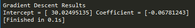
The R code for linear regression versus gradient descent is as follows:
# Linear Regression
train_data = read.csv("mtcars.csv",header=TRUE)
model <- lm(mpg ~ hp, data = train_data)
print (coef(model))

# Gradient descent
gradDesc <- function(x, y, learn_rate, conv_threshold, batch_size, max_iter) {
  m <- runif(1, 0, 1)
  c <- runif(1, 0, 1)
  ypred <- m * x + c
  MSE <- sum((y - ypred) ^ 2) / batch_size

  converged = F
  iterations = 0

  while(converged == F) {
    m_new <- m - learn_rate * ((1 / batch_size) * (sum((ypred - y) * x)))
    c_new <- c - learn_rate * ((1 / batch_size) * (sum(ypred - y)))

    m <- m_new
    c <- c_new
  ypred <- m * x + c
    MSE_new <- sum((y - ypred) ^ 2) / batch_size

    if(MSE - MSE_new <= conv_threshold) {
      converged = T
      return(paste("Iterations:",iterations,"Optimal intercept:", c, "Optimal slope:", m))
    }
    iterations = iterations + 1

    if(iterations > max_iter) {
      converged = T
      return(paste("Iterations:",iterations,"Optimal intercept:", c, "Optimal slope:", m))
    }
    MSE = MSE_new
  }
}
gradDesc(x = train_data$hp,y =  train_data$mpg, learn_rate = 0.00003, conv_threshold = 1e-8, batch_size = 32, max_iter = 1500000)
The loss function or cost function in machine learning is a function that maps the values of variables onto a real number intuitively representing some cost associated with the variable values. Optimization methods are applied to minimize the loss function by changing the parameter values, which is the central theme of machine learning.
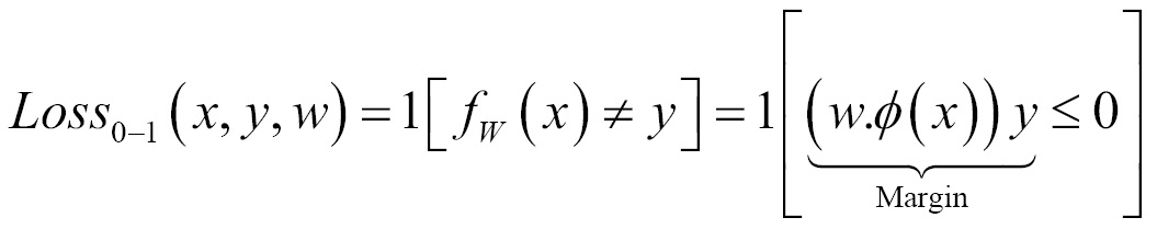
Zero-one loss is L0-1 = 1 (m <= 0); in zero-one loss, value of loss is 0 for m >= 0 whereas 1 for m < 0. The difficult part with this loss is it is not differentiable, non-convex, and also NP-hard. Hence, in order to make optimization feasible and solvable, these losses are replaced by different surrogate losses for different problems.
Surrogate losses used for machine learning in place of zero-one loss are given as follows. The zero-one loss is not differentiable, hence approximated losses are being used instead:
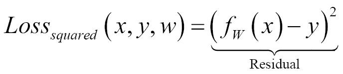
- Squared loss (for regression)
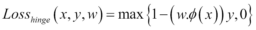
- Hinge loss (SVM)
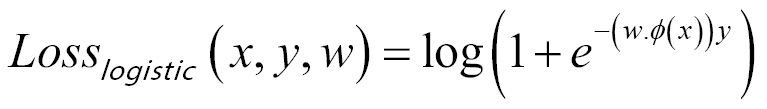
- Logistic/log loss (logistic regression)
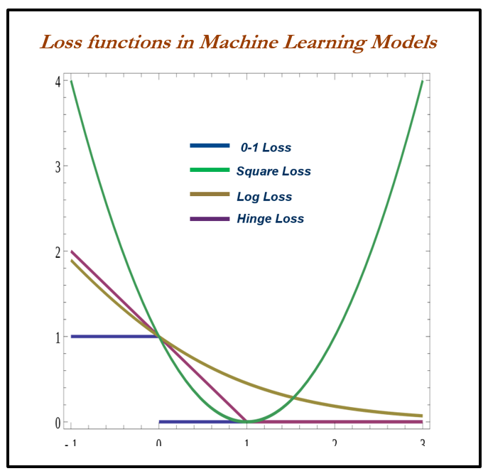
Some loss functions are as follows:
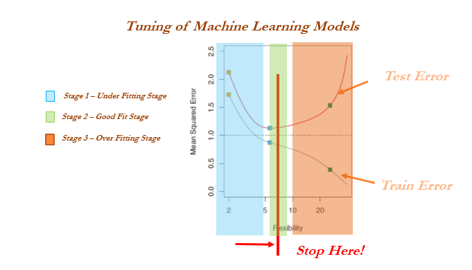
When to stop tuning the hyperparameters in a machine learning model is a million-dollar question. This problem can be mostly solved by keeping tabs on training and testing errors. While increasing the complexity of a model, the following stages occur:
- Stage 1: Underfitting stage - high train and high test errors (or low train and low test accuracy)
- Stage 2: Good fit stage (ideal scenario) - low train and low test errors (or high train and high test accuracy)
- Stage 3: Overfitting stage - low train and high test errors (or high train and low test accuracy)
Cross-validation is not popular in the statistical modeling world for many reasons; statistical models are linear in nature and robust, and do not have a high variance/overfitting problem. Hence, the model fit will remain the same either on train or test data, which does not hold true in the machine learning world. Also, in statistical modeling, lots of tests are performed at the individual parameter level apart from aggregated metrics, whereas in machine learning we do not have visibility at the individual parameter level:
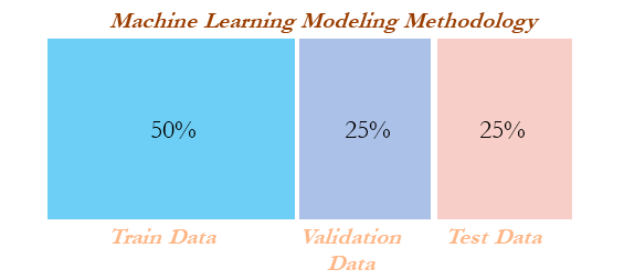
In the following code, both the R and Python implementation has been provided. If none of the percentages are provided, the default parameters are 50 percent for train data, 25 percent for validation data, and 25 percent for the remaining test data.
Python implementation has only one train and test split functionality, hence we have used it twice and also used the number of observations to split rather than the percentage (as shown in the previous train and test split example). Hence, a customized function is needed to split into three datasets:
>>> import pandas as pd
>>> from sklearn.model_selection import train_test_split

>>> original_data = pd.read_csv("mtcars.csv")

>>> def data_split(dat,trf = 0.5,vlf=0.25,tsf = 0.25):
...      nrows = dat.shape[0]
...      trnr = int(nrows*trf)
...      vlnr = int(nrows*vlf)
The following Python code splits the data into training and the remaining data. The remaining data will be further split into validation and test datasets:
...      tr_data,rmng = train_test_split(dat,train_size = trnr,random_state=42)
...      vl_data, ts_data = train_test_split(rmng,train_size = vlnr,random_state=45)
...      return (tr_data,vl_data,ts_data)
Implementation of the split function on the original data to create three datasets (by 50 percent, 25 percent, and 25 percent splits) is as follows:
>>> train_data, validation_data, test_data = data_split (original_data ,trf=0.5, vlf=0.25,tsf=0.25)The R code for the train, validation, and test split is as follows:
# Train Validation & Test samples
trvaltest <- function(dat,prop = c(0.5,0.25,0.25)){
  nrw = nrow(dat)
  trnr = as.integer(nrw *prop[1])
  vlnr = as.integer(nrw*prop[2])
  set.seed(123)
  trni = sample(1:nrow(dat),trnr)
  trndata = dat[trni,]
  rmng = dat[-trni,]
  vlni = sample(1:nrow(rmng),vlnr)
  valdata = rmng[vlni,]
  tstdata = rmng[-vlni,]
  mylist = list("trn" = trndata,"val"= valdata,"tst" = tstdata)
  return(mylist)
}
outdata = trvaltest(mtcars,prop = c(0.5,0.25,0.25))
train_data = outdata$trn; valid_data = outdata$val; test_data = outdata$tst
Cross-validation is another way of ensuring robustness in the model at the expense of computation. In the ordinary modeling methodology, a model is developed on train data and evaluated on test data. In some extreme cases, train and test might not have been homogeneously selected and some unseen extreme cases might appear in the test data, which will drag down the performance of the model.
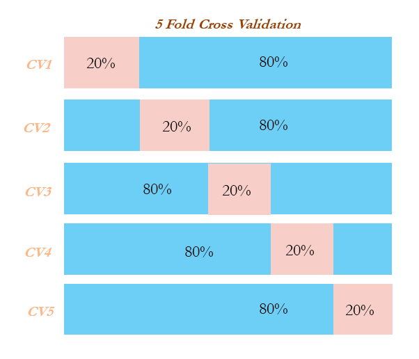
On the other hand, in cross-validation methodology, data was divided into equal parts and training performed on all the other parts of the data except one part, on which performance will be evaluated. This process repeated as many parts user has chosen.
Example: In five-fold cross-validation, data will be divided into five parts, subsequently trained on four parts of the data, and tested on the one part of the data. This process will run five times, in order to cover all points in the data. Finally, the error calculated will be the average of all the errors:
Grid search in machine learning is a popular way to tune the hyperparameters of the model in order to find the best combination for determining the best fit:
In the following code, implementation has been performed to determine whether a particular user will click an ad or not. Grid search has been implemented using a decision tree classifier for classification purposes. Tuning parameters are the depth of the tree, the minimum number of observations in terminal node, and the minimum number of observations required to perform the node split:
# Grid search
>>> import pandas as pd
>>> from sklearn.tree import DecisionTreeClassifier
>>> from sklearn.model_selection import train_test_split
>>> from sklearn.metrics import classification_report,confusion_matrix,accuracy_score
>>> from sklearn.pipeline import Pipeline
>>> from sklearn.grid_search import GridSearchCV

>>> input_data = pd.read_csv("ad.csv",header=None)

>>> X_columns = set(input_data.columns.values)
>>> y = input_data[len(input_data.columns.values)-1]
>>> X_columns.remove(len(input_data.columns.values)-1)
>>> X = input_data[list(X_columns)]
Split the data into train and testing:
>>> X_train, X_test,y_train,y_test = train_test_split(X,y,train_size = 0.7,random_state=33)Create a pipeline to create combinations of variables for the grid search:
>>> pipeline = Pipeline([
...      ('clf', DecisionTreeClassifier(criterion='entropy')) ])
Combinations to explore are given as parameters in Python dictionary format:
>>> parameters = {
...      'clf__max_depth': (50,100,150),
...      'clf__min_samples_split': (2, 3),
...      'clf__min_samples_leaf': (1, 2, 3)}
The n_jobs field is for selecting the number of cores in a computer; -1 means it uses all the cores in the computer. The scoring methodology is accuracy, in which many other options can be chosen, such as precision, recall, and f1:
>>> grid_search = GridSearchCV(pipeline, parameters, n_jobs=-1, verbose=1, scoring='accuracy')
>>> grid_search.fit(X_train, y_train)
Predict using the best parameters of grid search:
>>> y_pred = grid_search.predict(X_test)The output is as follows:
>>> print ('\n Best score: \n', grid_search.best_score_)
>>> print ('\n Best parameters set: \n')
>>> best_parameters = grid_search.best_estimator_.get_params()
>>> for param_name in sorted(parameters.keys()):
>>>     print ('\t%s: %r' % (param_name, best_parameters[param_name]))
>>> print ("\n Confusion Matrix on Test data \n",confusion_matrix(y_test,y_pred))
>>> print ("\n Test Accuracy \n",accuracy_score(y_test,y_pred))
>>> print ("\nPrecision Recall f1 table \n",classification_report(y_test, y_pred))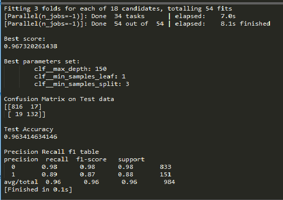
The R code for grid searches on decision trees is as follows:
# Grid Search on Decision Trees
library(rpart)
input_data = read.csv("ad.csv",header=FALSE)
input_data$V1559 = as.factor(input_data$V1559)
set.seed(123)
numrow = nrow(input_data)
trnind = sample(1:numrow,size = as.integer(0.7*numrow))

train_data = input_data[trnind,];test_data = input_data[-trnind,]
minspset = c(2,3);minobset = c(1,2,3)
initacc = 0

for (minsp in minspset){
  for (minob in minobset){
    tr_fit = rpart(V1559 ~.,data = train_data,method = "class",minsplit = minsp, minbucket = minob)
    tr_predt = predict(tr_fit,newdata = train_data,type = "class")
    tble = table(tr_predt,train_data$V1559)
    acc = (tble[1,1]+tble[2,2])/sum(tble)
    acc
    if (acc > initacc){
      tr_predtst = predict(tr_fit,newdata = test_data,type = "class")
      tblet = table(test_data$V1559,tr_predtst)
      acct = (tblet[1,1]+tblet[2,2])/sum(tblet)
      acct
      print(paste("Best Score"))
      print( paste("Train Accuracy ",round(acc,3),"Test Accuracy",round(acct,3)))
      print( paste(" Min split ",minsp," Min obs per node ",minob))
      print(paste("Confusion matrix on test data"))
      print(tblet)
      precsn_0 = (tblet[1,1])/(tblet[1,1]+tblet[2,1])
      precsn_1 = (tblet[2,2])/(tblet[1,2]+tblet[2,2])
      print(paste("Precision_0: ",round(precsn_0,3),"Precision_1: ",round(precsn_1,3)))
      rcall_0 = (tblet[1,1])/(tblet[1,1]+tblet[1,2])
      rcall_1 = (tblet[2,2])/(tblet[2,1]+tblet[2,2])
      print(paste("Recall_0: ",round(rcall_0,3),"Recall_1: ",round(rcall_1,3)))
      initacc = acc
    }
  }
}