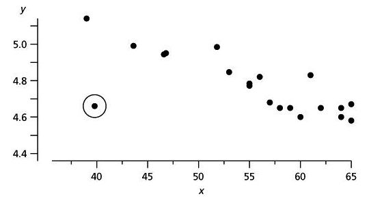
The goal of data preprocessing tasks is to prepare the data for a machine learning algorithm in the best possible way, as not all algorithms are capable of addressing issues with missing data, extra attributes, or denormalized values.

Data cleaning, also known as data cleansing or data scrubbing, is a process consisting of the following steps:

1. Identifying inaccurate, incomplete, irrelevant, or corrupted data to remove it from further processing
2. Parsing data, extracting information of interest, or validating whether a string of data is in an acceptable format
3. Transforming data into a common encoding format, for example, UTF-8 or int32, time scale, or a normalized range
4. Transforming data into a common data schema; for instance, if we collect temperature measurements from different types of sensors, we might want them to have the same structure

Machine learning algorithms generally do not work well with missing values. Rare exceptions include decision trees, Naive Bayes classifier, and some rule-based learners. It is very important to understand why a value is missing. It can be missing due to many reasons, such as random error, systematic error, and sensor noise. Once we identify the reason, there are multiple ways to deal with the missing values, as shown in the following list:

• Remove the instance: If there is enough data, and only a couple of non-relevant instances have some missing values, then it is safe to remove these instances.
• Remove the attribute: Removing an attribute makes sense when most of the values are missing, values are constant, or an attribute is strongly correlated with another attribute.
• Assign a special value (N/A): Sometimes a value is missing due to valid reasons, such as the value is out of scope, the discrete attribute value is not defined, or it is not possible to obtain or measure the value. For example, if a person never rates a movie, their rating on this movie is nonexistent.
• Take the average attribute value: If we have a limited number of instances, we might not be able to afford removing instances or attributes. In that case, we can estimate the missing values by assigning the average attribute value.
• Predict the value from other attributes: Predict the value from previous entries if the attribute possesses time dependencies.

As we have seen, the value can be missing for many reasons, and hence, it is important to understand why the value is missing, absent, or corrupted.

Outliers in data are values that are unlike any other values in the series and affect all learning methods to various degrees. These can be extreme values, which could be detected with confidence intervals and removed by using a threshold. The best approach is to visualize the data and inspect the visualization to detect irregularities. An example is shown in the following diagram. Visualization applies to low-dimensional data only:

Data transformation techniques tame the dataset to a format that a machine learning algorithm expects as input and may even help the algorithm to learn faster and achieve better performance. It is also known as data munging or data wrangling. Standardization, for instance, assumes that data follows Gaussian distribution and transforms the values in such a way that the mean value is 0 and the deviation is 1, as follows:

Normalization, on the other hand, scales the values of attributes to a small, specified range, usually between 0 and 1:

Many machine learning toolboxes automatically normalize and standardize the data for you.

The last transformation technique is discretization, which divides the range of a continuous attribute into intervals. Why should we care? Some algorithms, such as decision trees and Naive Bayes prefer discrete attributes. The most common ways to select the intervals are as follows:

• Equal width: The interval of continuous variables is divided into k equal width intervals
• Equal frequency: Supposing there are N instances, each of the k intervals contains approximately N or k instances
• Min entropy: This approach recursively splits the intervals until the entropy, which measures disorder, decreases more than the entropy increase, introduced by the interval split (Fayyad and Irani, 1993)

The first two methods require us to specify the number of intervals, while the last method sets the number of intervals automatically; however, it requires the class variable, which means it won't work for unsupervised machine learning tasks.

Data reduction deals with abundant attributes and instances. The number of attributes corresponds to the number of dimensions in our dataset. Dimensions with low prediction power contribute very little to the overall model, and cause a lot of harm. For instance, an attribute with random values can introduce some random patterns that will be picked up by a machine learning algorithm. It may happen that data contains a large number of missing values, wherein we have to find the reason for missing values in large numbers, and on that basis, it may fill it with some alternate value or impute or remove the attribute altogether. If 40% or more values are missing, then it may be advisable to remove such attributes, as this will impact the model performance.

The other factor is variance, where the constant variable may have low variance, which means the data is very close to each other or there is not very much variation in the data.

To deal with this problem, the first set of techniques removes such attributes and selects the most promising ones. This process is known as feature selection, or attributes selection, and includes methods such as ReliefF, information gain, and the Gini index. These methods are mainly focused on discrete attributes.

Another set of tools, focused on continuous attributes, transforms the dataset from the original dimensions into a lower-dimensional space. For example, if we have a set of points in three-dimensional space, we can make a projection into a two-dimensional space. Some information is lost, but in a situation where the third dimension is irrelevant, we don't lose much, as the data structure and relationships are almost perfectly preserved. This can be performed by the following methods:

• Singular value decomposition (SVD)
• Principal component analysis (PCA)
• Backward/forward feature elimination
• Factor analysis
• Linear discriminant analysis (LDA)
• Neural network autoencoders

The second problem in data reduction is related to too many instances; for example, they can be duplicates or come from a very frequent data stream. The main idea is to select a subset of instances in such a way that distribution of the selected data still resembles the original data distribution, and more importantly, the observed process. Techniques to reduce the number of instances involve random data sampling, stratification, and others. Once the data is prepared, we can start with the data analysis and modeling.