DNNs are ANNs which are strongly oriented to DL. Where normal procedures of analysis are inapplicable, due to the complexity of the data to be processed, such networks are therefore an excellent modeling tool. DNNs are neural networks that are very similar to those we have discussed, but they must implement a more complex model (a greater number of neurons, hidden layers, and connections), although they follow the learning principles that apply to all ML problems (such as supervised learning). The computation in each layer transforms the representations in the layer below into slightly more abstract representations.

We will use the term DNN to refer specifically to Multilayer Perceptron (MLP), Stacked Auto-Encoder (SAE), and Deep Belief Networks (DBNs). SAEs and DBNs use AutoEncoders (AEs) and RBMs as building blocks of the architectures. The main difference between them and MLP is that training is executed in two phases: unsupervised pre-training and supervised fine-tuning:

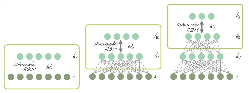
Figure 12: SAE and DBN using AE and RBM respectively.

In unsupervised pre-training, shown in the preceding diagram, the layers are stacked sequentially and trained in a layer-wise manner, like an AE or RBM using unlabeled data. Afterwards, in supervised fine-tuning, an output classifier layer is stacked, and the complete neural network is optimized, by retraining with labeled data.

In this chapter, we will not discuss SAEs (see more details in Chapter 5, Optimizing TensorFlow Autoencoders), but will stick to MLPs and DBNs and use these two DNN architectures. We will see how to develop predictive models to deal with high-dimensional datasets.

Multilayer perceptron

In multilayer networks, you can identify the artificial neurons of the layers, so that each neuron is connected to all those in the next layer, ensuring that:

• There are no connections between neurons belonging to the same layer

• There are no connections between neurons belonging to non-adjacent layers

• The number of layers and neurons per layer depends on the problem to be solved

The input and output layers define inputs and outputs, and there are hidden layers, whose complexity realizes different behaviors of the network. Finally, the connections between neurons are represented by as many matrices as the pairs of adjacent layers.

Each array contains the weights of the connections between the pairs of nodes of two adjacent layers. The feedforward networks are networks with no loops within the layers.

We will describe feedforward networks in more detail in Chapter 3, Feed-Forward Neural Networks with TensorFlow:

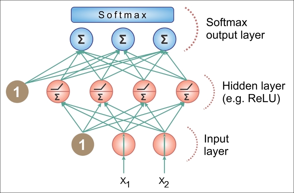
Figure 13: MLP architecture

Deep Belief Networks (DBNs)

To overcome the overfitting problem in MLP, we set up a DBN, do unsupervised pre-training to get a decent set of feature representations for the inputs, then fine-tune the training set to get actual predictions from the network. While the weights of an MLP are initialized randomly, a DBN uses a greedy layer-by-layer pre-training algorithm to initialize the network weights through probabilistic generative models. The models are composed of a visible layer and multiple layers of stochastic and latent variables, which are called hidden units or feature detectors.

DBNs are Deep Generative Models, which are neural network models that can replicate the data distribution that you provide. This allows you to generate "fake-but-realistic" data points from real data points.

DBNs are composed of a visible layer and multiple layers of stochastic, latent variables, which are called hidden units or feature detectors. The top two layers have undirected, symmetric connections between them and form an associative memory, whereas lower layers receive top-down, directed connections from the preceding layer. The building blocks of DBNs are Restricted Boltzmann Machines (RBMs). As you can see in the following figure, several RBMs are stacked one after another to form DBNs:

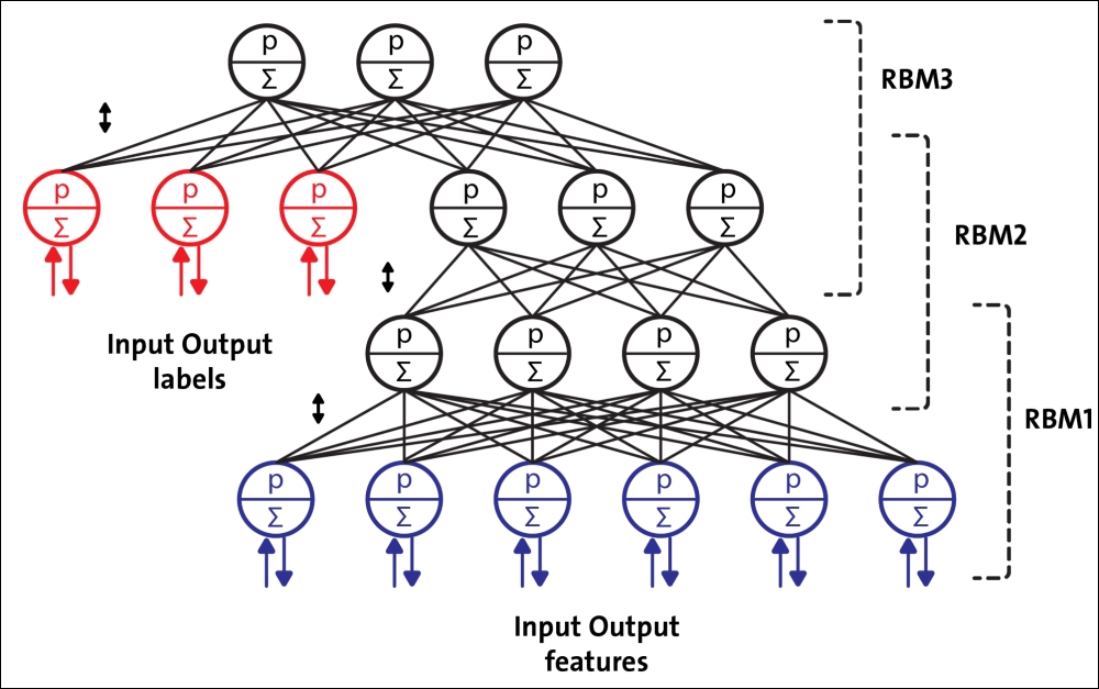
Figure 14: A DBN configured for semi-supervised learning

A single RBM consists of two layers. The first layer is composed of visible neurons, and the second layer consists of hidden neurons. The following figure shows the structure of a simple RBM. Visible units accept inputs, and hidden units are nonlinear feature detectors. Each visible neuron is connected to all the hidden neurons, but there is no internal connection among neurons in the same layer.

An RBM consists of a visible layer node and a hidden layer node, but without visible-visible and hidden-hidden connections, hence the term restricted. They allow more efficient network training that can be supervised or unsupervised. This type of neural network is able to represent a large number of features of the inputs, then hidden nodes can represent up to 2n features. The network can be trained to respond to a single question (for example, yes or no to the question: Is it a cat?) until it can respond (again in binary terms) to a total of 2n questions (Is it a cat?, It is Siamese?, Is it white?).

The architecture of the RBM is as follows, with neurons arranged according to a symmetrical bipartite graph:

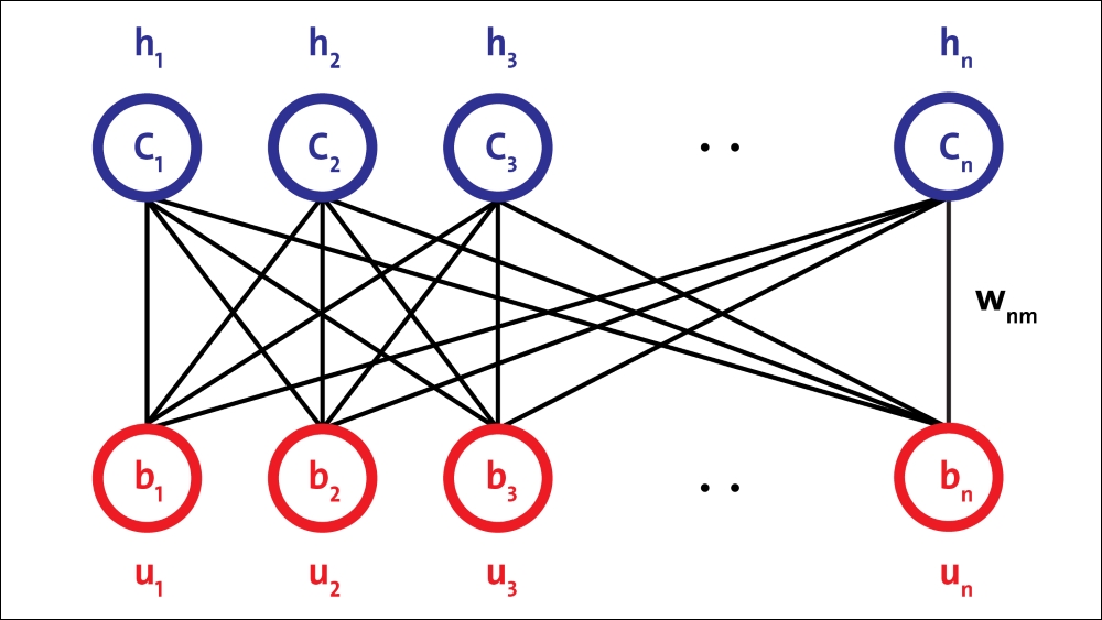
Figure 15: RBM architecture.

A single hidden layer RBM cannot extract all the features from the input data, due to its inability to model the relationship between variables. Hence, multiple layers of RBMs are used one after another to extract nonlinear features. In DBNs, an RBM is trained first with input data, and the hidden layer represents the features learned using a greedy learning approach. These learned features of the first RBM, that is, a hidden layer of the first RBM, are used as the input to the second RBM, as another layer in the DBN.

Similarly, the learned features of the second layer are used as input for another layer. This way, DBNs can extract deep and nonlinear features from input data. The hidden layer of the last RBM represents the learned features of the whole network.

CNNs have been specifically designed for image recognition. Each image used in learning is divided into compact topological portions, each of which will be processed by filters to search for particular patterns. Formally, each image is represented as a three-dimensional matrix of pixels (width, height, and color), and every sub-portion can be placed on convolution with the filter set. In other words, scrolling each filter along the image computes the inner product of the same filter and input.

This procedure produces a set of feature maps (activation maps) for the various filters. Superimposing the various feature maps onto the same portion of the image, we get an output volume. This type of layer is called the convolutional layer. The following diagram is a schematic of the architecture of a CNN:

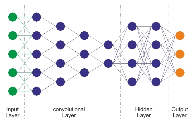
Figure 16: CNN architecture.

Although regular DNNs work fine for small images (for example, MNIST and CIFAR-10), they break down with larger images because of the huge number of parameters required. For example, a 100×100 image has 10,000 pixels, and if the first layer has just 1,000 neurons (which already severely restricts the amount of information transmitted to the next layer), this means 10 million connections. In addition, that is just for the first layer.

CNNs solve this problem using partially connected layers. Because consecutive layers are only partially connected and because it heavily reuses its weights, a CNN has far fewer parameters than a fully connected DNN, which makes it much faster to train. This reduces the risk of overfitting and requires much less training data. Moreover, when a CNN has learned a kernel that can detect a particular feature, it can detect that feature anywhere on the image. In contrast, when a DNN learns a feature in one location, it can detect it only in that particular location. Since images typically have very repetitive features, CNNs are able to generalize much better than DNNs on image processing tasks such as classification and use fewer training examples.

Importantly, the DNN has no prior knowledge of how the pixels are organized; it does not know that nearby pixels are close. A CNN's architecture embeds this prior knowledge. Lower layers typically identify features in small areas of the images, while higher layers combine the lower-level features into larger features. This works well with most natural images, giving CNNs a decisive head-start over DNNs:

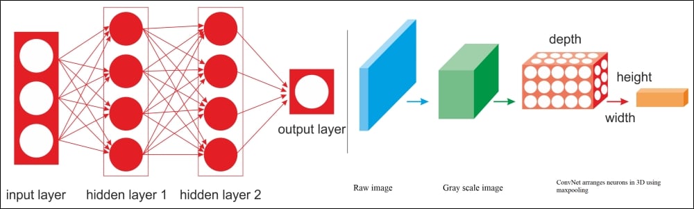
Figure 17: A regular DNN versus a CNN.

For example, in the preceding diagram, on the left, you can see a regular three-layer neural network. On the right, a CNN arranges its neurons in three dimensions (width, height, and depth), as visualized in one of the layers. Every layer of a CNN transforms the 3D input volume to a 3D output volume of neuron activations. The red input layer holds the image, so its width and height would be the dimensions of the image, and the depth would be three (red, green and blue channels).

Therefore, all the multilayer neural networks we looked at had layers composed of a long line of neurons, and we had to flatten input images or data to 1D before feeding them to the neural network. However, what happens when you try to feed them a 2D image directly? The answer is that in a CNN, each layer is represented in 2D, which makes it easier to match neurons with their corresponding inputs. We will see examples of this in upcoming sections.

An AE is a network with three or more layers, where the input layer and the output have the same number of neurons, and those intermediate (hidden layers) have a lower number of neurons. The network is trained to simply reproduce in the output, for each piece of input data, the same pattern of activity in the input.

AEs are ANNs capable of learning efficient representations of the input data without any supervision (that is, the training set is unlabeled). They typically have a much lower dimensionality than the input data, making AEs useful for dimensionality reduction. More importantly, AEs act as powerful feature detectors, and they can be used for unsupervised pre-training of DNNs.

The remarkable aspect of the problem is that, due to the lower number of neurons in the hidden layer, if the network can learn from examples and generalize to an acceptable extent, it performs data compression; the status of the hidden neurons provides, for each example, a compressed version of the input and output common states. Useful applications of AEs are data denoising and dimensionality reduction for data visualization.

The following diagram shows how an AE typically works; it reconstructs the received input through two phases: an encoding phase, which corresponds to a dimensional reduction for the original input, and a decoding phase, which is capable of reconstructing the original input from the encoded (compressed) representation:

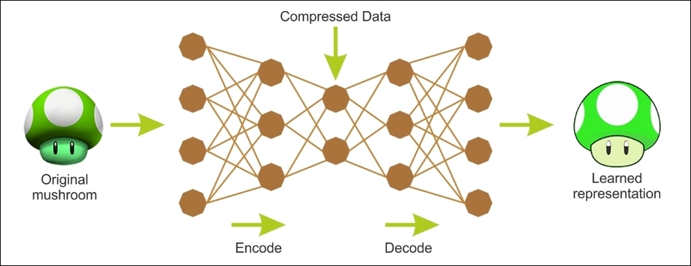
Figure 18: Encoding and decoding phases of an autoencoder.

As an unsupervised neural network, the main characteristic of an autoencoder is its symmetrical structure. An autoencoder has two components: an encoder that converts the input to an internal representation, followed by a decoder that converts the internal representation to the output.

In other words, an autoencoder can be seen as a combination of an encoder, where we encode some input into a code, and a decoder, where we decode/reconstruct the code back to its original input as the output. Thus, an MLP typically has the same architecture as an autoencoder, except that the number of neurons in the output layer must be equal to the number of inputs.

As mentioned previously, there is more than one way to train an autoencoder. The first way is to train the whole layer at once, similar to MLP. However, instead of using some labeled output when calculating the cost function, as in supervised learning, we use the input itself. Therefore, the cost function shows the difference between the actual input and the reconstructed input.

The fundamental feature of an RNN is that the network contains at least one feedback connection, so the activations can flow around in a loop. It enables the networks to do temporal processing and learn sequences, for example performing sequence recognition/reproduction or temporal association/prediction.

RNN architectures can have many different forms. One common type consists of a standard MLP plus added loops. These can exploit the powerful non-linear mapping capabilities of the MLP, and have some form of memory. Others have more uniform structures, potentially with every neuron connected to all the others, and may have stochastic activation functions:

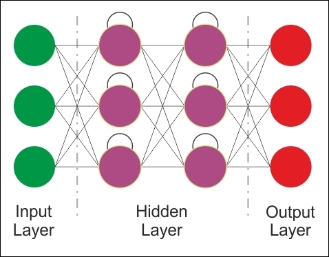
Figure 19: RNN architecture.

For simple architectures and deterministic activation functions, learning can be achieved using similar GD procedures to those leading to the backpropagation algorithm for feedforward networks.

The preceding image looks at a few of the most important types and features of RNNs. RNNs are designed to utilize sequential information of input data with cyclic connections among building blocks such as perceptrons, Long Short-term memory units (LSTMs), or Gated Recurrent units (GRUs). The latter two are used to remove the drawbacks of regular RNNs, such as the gradient vanishing/exploding problem and long-short term dependency. We will look at these architectures in later chapters.

Many other emergent DL architectures have been suggested, such as Deep SpatioTemporal Neural Networks (DST-NNs), Multi-Dimensional Recurrent Neural Networks (MD-RNNs), and Convolutional AutoEncoders (CAEs).

Nevertheless, people are talking about and using other emerging networks, such as CapsNets (an improved version of a CNN, designed to remove the drawbacks of regular CNNs), Factorization Machines for personalization, and Deep Reinforcement Learning.