

When you are working with huge arrays in machine learning projects, you often need to index, slice, reshape, and resize.
Indexing is a fundamental term used in mathematics and computer science. As a general term, indexing helps you to specify how to return desired elements of various data structures. The following example shows indexing for a list and a tuple:
In [74]: x = ["USA","France", "Germany","England"]
         x[2]
Out[74]: 'Germany'
In [75]: x = ('USA',3,"France",4)
         x[2]
Out[75]: 'France'
In NumPy, the main usage of indexing is controlling and manipulating the elements of arrays. It's a way of creating generic lookup values. Indexing contains three child operations, which are field access, basic slicing, and advanced indexing. In field access, you just specify the index of an element in an array to return the value for a given index.
NumPy is very powerful when it comes to indexing and slicing. In many cases, you need to refer your desired element in an array and do the operations on this sliced area. You can index your array similarly to what you do with tuples or lists with square bracket notations. Let's start with field access and simple slicing with one-dimensional arrays and move on to more advanced techniques:
In [76]: x = np.arange(10)
         x
Out[76]: array([0, 1, 2, 3, 4, 5, 6, 7, 8, 9])
In [77]: x[5]
Out[77]: 5
In [78]: x[-2]
Out[78]: 8
In [79]: x[2:8]
Out[79]: array([2, 3, 4, 5, 6, 7])
In [80]: x[:]
Out[80]: array([0, 1, 2, 3, 4, 5, 6, 7, 8, 9])
In [81]: x[2:8:2]
Out[81]: array([2, 4, 6])
Indexing starts from 0, so when you create an array with an element, your first element is indexed as x[0], the same way as your last element, x[n-1]. As you can see in the preceding example, x[5] refers to the sixth element. You can also use negative values in indexing. NumPy understands these values as the nth orders backwards. Like in the example, x[-2] refers to the second to last element. You can also select multiple elements in your array by stating the starting and ending indexes and also creating sequential indexing by stating the increment level as a third argument, as in the last line of the code.
So far, we have seen indexing and slicing in 1D arrays. The logic does not change, but for the sake of demonstration, let's do some practice for multidimensional arrays as well. The only thing that changes when you have multidimensional arrays is just having more axis. You can slice the n-dimensional array as [slicing in x-axis, slicing in y-axis] in the following code:
In [82]: x = np.reshape(np.arange(16),(4,4))
         x
Out[82]: array([[ 0, 1, 2, 3],
                [ 4, 5, 6, 7],
                [ 8, 9, 10, 11],
                [12, 13, 14, 15]])
In [83]: x[1:3]
Out[83]: array([[ 4, 5, 6, 7],
                [ 8, 9, 10, 11]])
In [84]: x[:,1:3]
Out[84]: array([[ 1, 2],
                [ 5, 6],
                [ 9, 10],
                [13, 14]])
In [85]: x[1:3,1:3]
Out[85]: array([[ 5, 6],
                [ 9, 10]])
You sliced the arrays row and column-wise, but you haven't sliced the elements in a more irregular or more dynamic fashion, which means you always slice them in a rectangular or square way. Imagine a 4*4 array that we want to slice as follows:
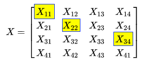
To obtain the preceding slicing, we execute the following code:
In [86]: x = np.reshape(np.arange(16),(4,4))
         x
Out[86]: array([[ 0, 1, 2, 3],
                [ 4, 5, 6, 7],
                [ 8, 9, 10, 11],
                [12, 13, 14, 15]])
In [87]: x[[0,1,2],[0,1,3]]
Out[87]: array([ 0, 5, 11])
In advanced indexing, the first part indicates the index of rows to be sliced and the second part indicates the corresponding columns. In the preceding example, you first sliced the 1st, 2nd, and 3rd rows ([0,1,2]) and then sliced the 1st, 2nd and 4th columns ([0,1,3]) into sliced rows.
The reshape and resize methods may seem similar, but there are differences in the outputs of these operations. When you reshape the array, it's just the output that changes the shape of the array temporarily, but it does not change the array itself. When you resize the array, it changes the size of the array permanently, and if the new array's size is bigger than the old one, the new array elements will be filled with repeated copies of the old ones. On the contrary, if the new array is smaller, a new array will take the elements from the old array with the order of index which is required to fill the new one. Please note that same data can be shared by different ndarrays which means that an ndarray can be a view to another ndarray. In such cases changes made in one array will have consequences on other views.
The following code gives an example of how the new array elements are filled when the size is bigger or smaller than the original array:
In [88]: x = np.arange(16).reshape(4,4)
         x
Out[88]: array([[ 0, 1, 2, 3],
                [ 4, 5, 6, 7],
                [ 8, 9, 10, 11],
                [12, 13, 14, 15]])
In [89]: np.resize(x,(2,2))
Out[89]: array([[0, 1],
                 [2, 3]])
In [90]: np.resize(x,(6,6))
Out[90]: array([[ 0, 1, 2, 3, 4, 5],
                [ 6, 7, 8, 9, 10, 11],
                [12, 13, 14, 15, 0, 1],
                [ 2, 3, 4, 5, 6, 7],
                [ 8, 9, 10, 11, 12, 13],
                [14, 15, 0, 1, 2, 3]])
The last important term of this subsection is broadcasting, which explains how NumPy behaves in arithmetic operations of the array when they have different shapes. NumPy has two rules for broadcasting: either the dimensions of the arrays are equal, or one of them is 1. If one of these conditions is not met, then you will get one of the two errors: frames are not aligned or operands could not be broadcast together:
In [91]: x = np.arange(16).reshape(4,4)
         y = np.arange(6).reshape(2,3)
         x+y
        ---------------------------------------------------------------                           ------------
        ValueError Traceback (most recent call last)
        <ipython-input-102-083fc792f8d9> in <module>()
        1 x = np.arange(16).reshape(4,4)
        2 y = np.arange(6).reshape(2,3)
        ----> 3 x+y
        12
        ValueError: operands could not be broadcast together with                      shapes (4,4) (2,3)
You might have seen that you can multiply two matrices with shapes (4, 4) and (4,) or with (2, 2) and (2, 1). The first case meets the condition of having one dimension so that the multiplication becomes a vector * array, which does not cause any broadcasting problems:
In [92]: x = np.ones(16).reshape(4,4)
          y = np.arange(4)
          x*y
Out[92]: array([[ 0., 1., 2., 3.],
                 [ 0., 1., 2., 3.],
                 [ 0., 1., 2., 3.],
                 [ 0., 1., 2., 3.]])
In [93]: x = np.arange(4).reshape(2,2)
         x
Out[93]: array([[0, 1],
                [2, 3]])
In [94]: y = np.arange(2).reshape(1,2)
         y
Out[94]: array([[0, 1]])
In [95]: x*y
Out[95]: array([[0, 1],
                [0, 3]])
The preceding code block gives an example for the second case, where during computation small arrays iterate through the large array and the output is stretched across the whole array. That's the reason why there are (4, 4) and (2, 2) outputs: during the multiplication, both arrays are broadcast to larger dimensions.