Neural networks

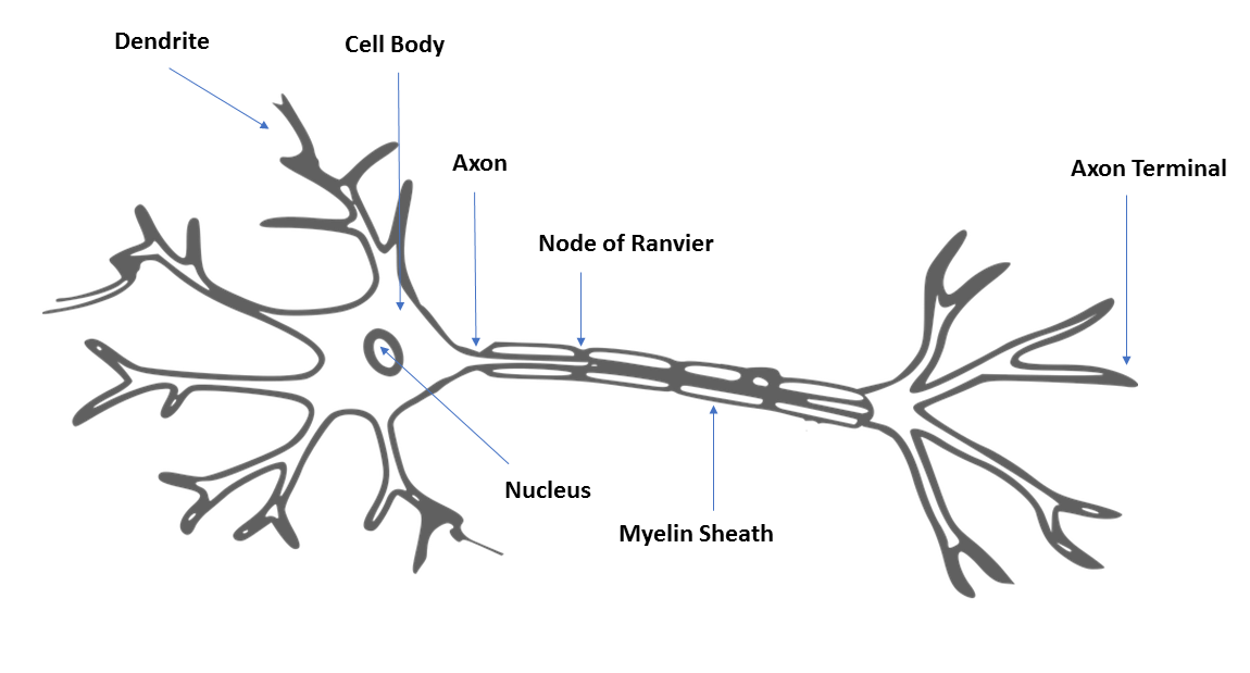
Neural networks are machine learning models that are inspired by the human brain. They consist of neural processing units they are interconnected with one another in a hierarchical fashion. These neural processing units are called artificial neurons, and they perform the same function as axons in a human brain. In a human brain, dendrites receive input from neighboring neurons, and attenuate or magnify the input before transmitting it on to the soma of the neuron. In the soma of the neuron, these modified signals are added together and passed on to the axon of the neuron. If the input to the axon is over a specified threshold, then the signal is passed on to the dendrites of the neighboring neurons.

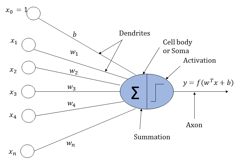
An artificial neuron loosely works perhaps on the same logic as that of a biological neuron. It receives input from neighboring neurons. The input is scaled by the input connections of the neurons and then added together. Finally, the summed input is passed through an activation function whose output is passed on to the neurons in the next layer.

A biological neuron and an artificial neuron are illustrated in the following diagrams for comparison:

An artificial neuron are illustrated in the following diagram:

Now, let's look at the structure of an artificial neural network, as illustrated in the following diagram:

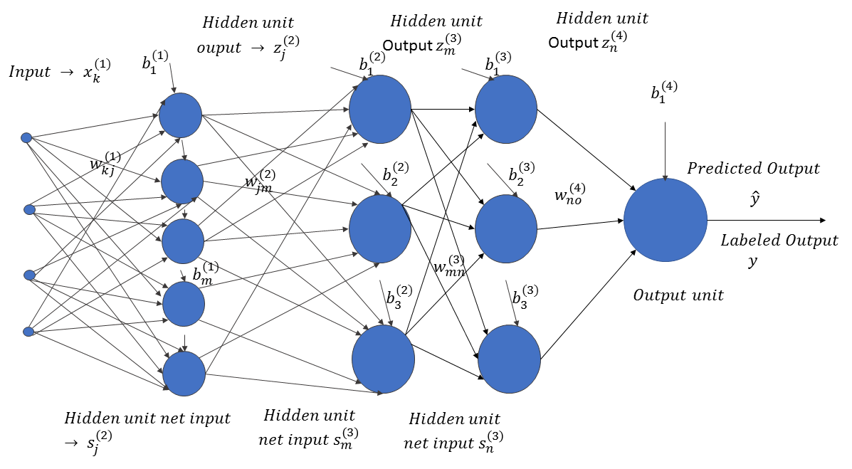
The input, x ∈ R^N, passes through successive layers of neural units, arranged in a hierarchical fashion. Each neuron in a specific layer receives an input from the neurons of the preceding layers, attenuated or amplified by the weights of the connections between them. The weight, , corresponds to the weight connection between the i^th neuron in layer l and the j^th neuron in layer (l+1). Also, each neuron unit, i, in a specific layer, l, is accompanied by a bias, . The neural network predicts the output, , for the input vector, x ∈ R^N. If the actual label of the data is y, where y takes continuous values, then the neuron network learns the weights and biases by minimizing the prediction error, . Of course, the error has to be minimized for all of the labeled data points: (x_i, y_i)∀_i ∈ 1, 2, . . . m.

If we denote the set of weights and biases by one common vector, W, and the total error in the prediction is represented by C, then through the training process, the estimated W can be expressed as follows:

Also, the predicted output, , can be represented by a function of the input, x, parameterized by the weight vector, W, as follows:

Such a formula for predicting the continuous values of the output is called a regression problem.

For a two-class binary classification, cross-entropy loss is minimized instead of the squared error loss, and the network outputs the probability of the positive class instead of the output. The cross-entropy loss can be represented as follows:

Here, p_i is the predicted probability of the output class, given the input x, and can be represented as a function of the input, x, parameterized by the weight vector, as follows:

In general, for multi-class classification problems (say, of n classes), the cross-entropy loss is given via the following:

Here, is the output label of the j^th class, for the i^th datapoint.