To train our model, we must define something called a loss function. The loss function will tell us how well or badly our model is currently doing its job.

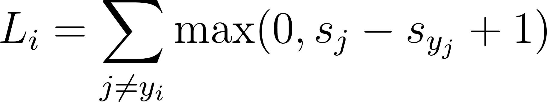
Losses can be found in the tf.losses module. For this model, we will use the hinge loss. Hinge loss is the loss function used when creating a support vector machine (SVM). Hinge loss heavily punishes incorrect predictions. For one given example,

, where

is a feature vector of a datapoint and

is its label, the hinge loss for it will be as follows:

To this, the following will apply:

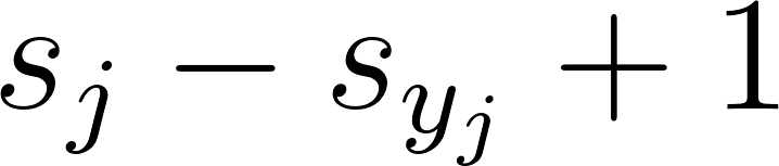
In simple words, this equation takes the raw output of the classifier. In our model, that's three output scores, and ensures that the score of the target class is greater, by at least 1, than the scores of the other classes. For each score (except the target class), if this restriction is satisfied, then 0 is added to the loss, otherwise, there's a penalty that is added:

This concept is actually very intuitive because if our weights and biases are trained properly, then the highest of the three produced scores should confidently indicate the correct class that an input example belongs to.

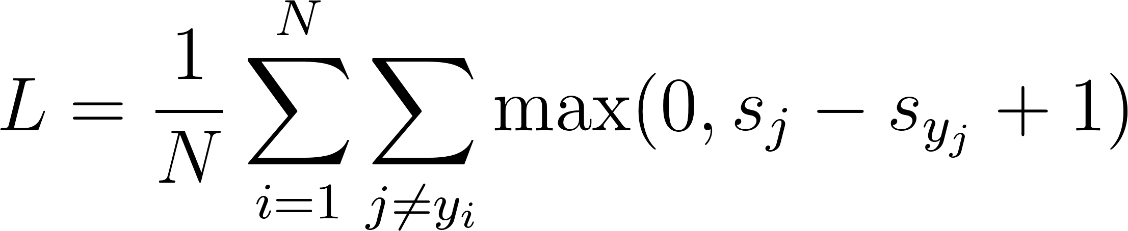
Since during training we feed many training examples in at once, we'll obtain multiple losses like these that need to be averaged. Therefore, the total loss equation that needs to be minimized is as follows:

In our code, the loss function will take two arguments: logits and labels. In TensorFlow, logits is the name for the raw values produced by our model. In our case, this is model_out as this is the output of our model. For labels, we use our label placeholder, y. Remember that the placeholder will be filled for us at runtime:

loss = tf.reduce_mean(tf.losses.hinge_loss(logits=model_out, labels=y))

As we also want to average our loss across the whole batch of input data, so we use tf.reduce_mean to average all our losses into one loss value that we will minimize.

There are many different types of lossfunctions available for us to use that are all good for different machine learning tasks. As we go through the book, we will learn more of them and when to use different loss functions.

Now we have defined a loss function to be used; we can use this loss function to train our model. As is shown in the previous equations, the loss function is a function of weights and biases. Therefore, all we have to do is an exhaustive search of the space of weights and biases and see which combination minimizes the loss best. When we have one- or two-dimensional weight vectors, this process might be okay, but when the weight vector space gets too big, we need a more efficient solution. To do this, we will use an optimization technique called gradient descent.

By using our loss function and calculus, gradient descent is able to see how to adjust the values of the weights and biases of our model in such a way that the value of the loss decreases. It is an iterative process requiring many iterations before the values of our weights and biases are well-adjusted for our training data. The idea is that the loss function L, parametrized by weights w, is minimized by updating the parameters in the opposite direction of the gradient of the objective function

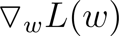
 with respect to the parameters. The update functions for weights and biases look like the following:

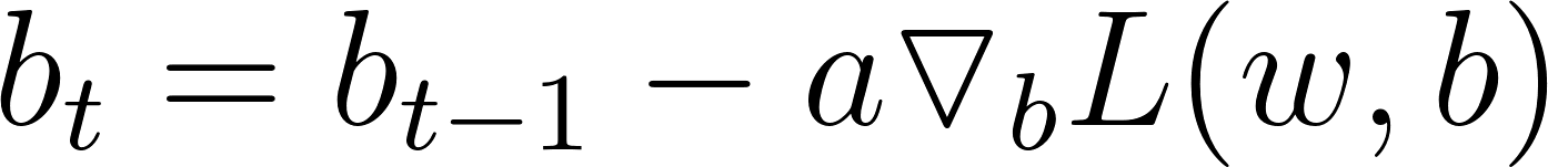
Here,

is the iteration number and

is a hyperparameter called the learning rate.

A loss function that is parameterized by two variables w1 and w2 will look something like in the following diagram:

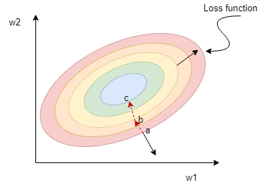
The preceding diagram shows the level curves of an elliptical paraboloid. This is a bowl-shaped surface and the bottom of the bowl lies at the center. Looking at the plot, the gradient vector at point a (the straight black arrow) is normal to the level curve through a. The gradient vector, in fact, points in the direction of the greatest rate of increase of the loss function.

So, if we start from point a and update the weights toward the direction opposite to the gradient vector, then we will descend to point b and in the next iteration to point c, and so on until we reach the minimum. The parameters that minimize the loss function are selected to represent the final trained linear model.

The nice thing about TensorFlow is it calculates all the required gradients for us using its built-in optimizers with something called automatic differentiation. All we have to do is choose a gradient descent optimizer and tell it to minimize our loss function. TensorFlow will automatically calculate all the gradients and then use these to update our weights for us.

We can find optimizer classes in the tf.train module. For now, we will use the GradientDescentOptimizer class, which is just the basic gradient descent optimization algorithm. When creating the optimizer, we must supply a learning rate. The value of the learning rate is a hyperparameter that the user must tune through trial and error and experimentation. The value of 0.5 should work well in this problem.

The optimizer node has a method called minimize. Calling this method on a loss function that you supply will do two things. First, gradients with respect to this loss are calculated for your whole graph. Second, these gradients are used to update all relevant variables.

Creating our optimizer node will look something like this:

optimizer = tf.train.GradientDescentOptimizer(learning_rate=0.5).minimize(loss) 

Like with loss functions, there are many different flavors of gradient descent optimizers to learn about. Presented here is the most basic kind, but again, we will learn about and use different ones in future chapters.