Activation functions are the key for neural networks to approximate non-linear outputs and adapt to non-linear features. They introduce non-linear operations into neural networks. If we are careful as to which activation functions are selected and where we put them, they are very powerful operations that we can tell TensorFlow to fit and optimize.

When we start to use neural networks, we will use activation functions regularly because activation functions are an essential part of any neural network. The goal of an activation function is just to adjust weight and bias. In TensorFlow, activation functions are non-linear operations that act on tensors. They are functions that operate in a similar way to the previous mathematical operations. Activation functions serve many purposes, but the main concept is that they introduce a non-linearity into the graph while normalizing the outputs. Start a TensorFlow graph with the following commands:

import tensorflow as tf 
sess = tf.Session() 

The activation functions live in the neural network (nn) library in TensorFlow. Besides using built-in activation functions, we can also design our own using TensorFlow operations. We can import the predefined activation functions (import tensorflow.nn as nn) or be explicit and write nn in our function calls. Here, we choose to be explicit with each function call:

1. The rectified linear unit, known as ReLU, is the most common and basic way to introduce non-linearity into neural networks. This function is just called max(0,x). It is continuous, but not smooth. It appears as follows:

print(sess.run(tf.nn.relu([-3., 3., 10.]))) 
[  0.  3.  10.] 

2. There are times where we will want to cap the linearly increasing part of the preceding ReLU activation function. We can do this by nesting the max(0,x) function into a min() function. The implementation that TensorFlow has is called the ReLU6 function. This is defined as min(max(0,x),6). This is a version of the hard-sigmoid function and is computationally faster, and does not suffer from vanishing (infinitesimally near zero) or exploding values. This will come in handy when we discuss deeper neural networks in Chapter 8, Convolutional Neural Networks, and Chapter 9, Recurrent Neural Networks. It appears as follows:

print(sess.run(tf.nn.relu6([-3., 3., 10.]))) 
[ 0. 3. 6.]

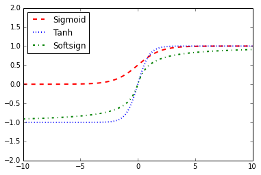
3. The sigmoid function is the most common continuous and smooth activation function. It is also called a logistic function and has the form . The sigmoid function is not used very often because of its tendency to zero-out the backpropagation terms during training. It appears as follows:

print(sess.run(tf.nn.sigmoid([-1., 0., 1.]))) 
[ 0.26894143  0.5         0.7310586 ] 

4. Another smooth activation function is the hyper tangent. The hyper tangent function is very similar to the sigmoid except that instead of having a range between 0 and 1, it has a range between -1 and 1. This function has the form of the ratio of the hyperbolic sine over the hyperbolic cosine. Another way to write this is . This activation function is as follows:

print(sess.run(tf.nn.tanh([-1., 0., 1.]))) 
[-0.76159418  0.         0.76159418 ] 

5. The softsign function also gets used as an activation function. The form of this function is . The softsign function is supposed to be a continuous (but not smooth) approximation to the sign function. See the following code:

print(sess.run(tf.nn.softsign([-1., 0., -1.]))) 
[-0.5  0.   0.5] 

6. Another function, the softplus function, is a smooth version of the ReLU function. The form of this function is . It appears as follows:

print(sess.run(tf.nn.softplus([-1., 0., -1.]))) 
[ 0.31326166  0.69314718  1.31326163] 

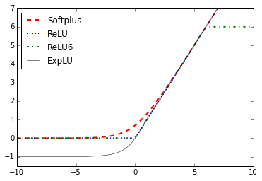
7. The Exponential Linear Unit (ELU) is very similar to the softplus function except that the bottom asymptote is -1 instead of 0. The form is if x < 0 else x. It appears as follows:

print(sess.run(tf.nn.elu([-1., 0., -1.]))) 
[-0.63212055  0.          1.        ] 

These activation functions are ways that we can introduce non-linearities in neural networks or other computational graphs in the future. It is important to note where in our network we are using activation functions. If the activation function has a range between 0 and 1 (sigmoid), then the computational graph can only output values between 0 and 1. If the activation functions are inside and hidden between nodes, then we want to be aware of the effect that the range can have on our tensors as we pass them through. If our tensors were scaled to have a mean of zero, we will want to use an activation function that preserves as much variance as possible around zero. This would imply that we want to choose an activation function such as the hyperbolic tangent (tanh) or the softsign. If the tensors are all scaled to be positive, then we would ideally choose an activation function that preserves variance in the positive domain.

Here are two graphs that illustrate the different activation functions. The following graphs show the ReLU, ReLU6, softplus, exponential LU, sigmoid, softsign, and hyperbolic tangent functions:

Here, we can see four of the activation functions: softplus, ReLU, ReLU6, and exponential LU. These functions flatten out to the left of zero and linearly increase to the right of zero, with the exception of ReLU6, which has a maximum value of six:

Here are the sigmoid, hyperbolic tangent (tanh), and softsign activation functions. These activation functions are all smooth and have a S n shape. Note that there are two horizontal asymptotes for these functions.