Training stability is one of the biggest problems that occur concerning GANs. For some datasets, GANs never converge due to this type of problem. In this section, we will look at some solutions that we can use to improve the stability of GANs.

During the training of GANs, we maximize the objective function of the discriminator network and minimize the objective function of the generator network. This objective function has some serious flaws. For example, it doesn't take into account the statistics of the generated data and the real data.

Feature matching is a technique that was proposed by Tim Salimans, Ian Goodfellow, and others in their paper titled Improved Techniques for Training GANs, to improve the convergence of the GANs by introducing a new objective function. The new objective function for the generator network encourages it to generate data, with statistics, that is similar to the real data.

To apply feature mapping, the network doesn't ask the discriminator to provide binary labels. Instead, the discriminator network provides activations or feature maps of the input data, extracted from an intermediate layer in the discriminator network. From a training perspective, we train the discriminator network to learn the important statistics of the real data; hence, the objective is that it should be capable of discriminating the real data from the fake data by learning those discriminative features.

To understand this approach mathematically, let's take a look at the different notations first:

• : The activation or feature maps for the real data from an intermediate layer in the discriminator network
• : The activation/feature maps for the data generated by the generator network from an intermediate layer in the discriminator network

This new objective function can be represented as follows:

Using this objective function can achieve better results, but there is still no guarantee of convergence.

Mini-batch discrimination is another approach to stabilize the training of GANs. It was proposed by Ian Goodfellow and others in Improved Techniques for Training GANs, which is available at https://arxiv.org/pdf/1606.03498.pdf. To understand this approach, let's first look in detail at the problem. While training GANs, when we pass the independent inputs to the discriminator network, the coordination between the gradients might be missing, and this prevents the discriminator network from learning how to differentiate between various images generated by the generator network. This is mode collapse, a problem we looked at earlier. To tackle this problem, we can use mini-batch discrimination. The following diagram illustrates the process very well:

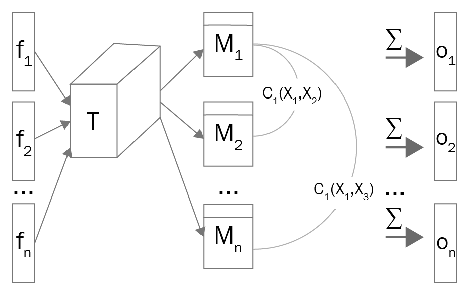
Mini-batch discrimination is a multi-step process. Perform the following steps to add mini-batch discrimination to your network:

1. Extract the feature maps for the sample and multiply them by a tensor, , generating a matrix, .
2. Then, calculate the L1 distance between the rows of the matrix using the following equation:

3. Then, calculate the summation of all distances for a particular example, :

3. Then, concatenate with and feed it to the next layer of the network:

To understand this approach mathematically, let's take a closer look at the various notions:

• : The activation or feature maps for sample from an intermediate layer in the discriminator network
• : A three-dimensional tensor, which we multiply by
• : The matrix generated when we multiply the tensor T and
• : The output after taking the sum of all distances for a particular example,

Mini-batch discrimination helps prevent mode collapse and improves the chances of training stability.

Historical averaging is an approach that takes the average of the parameters in the past and adds this to the respective cost functions of the generator and the discriminator network. It was proposed by Ian Goodfellow and others in a paper mentioned previously, Improved Techniques for Training GANs.

The historical average can be denoted as follows:

In the preceding equation, is the value of parameters at a particular time, i. This approach can improve the training stability of GANs too.

Earlier, label/target values for a classifier were 0 or 1; 0 for fake images and 1 for real images. Because of this, GANs were prone to adversarial examples, which are inputs to a neural network that result in an incorrect output from the network. Label smoothing is an approach to provide smoothed labels to the discriminator network. This means we can have decimal values such as 0.9 (true), 0.8 (true), 0.1 (fake), or 0.2 (fake), instead of labeling every example as either 1 (true) or 0 (fake). We smooth the target values (label values) of the real images as well as of the fake images. Label smoothing can reduce the risk of adversarial examples in GANs. To apply label smoothing, assign the labels 0.9, 0.8, and 0.7, and 0.1, 0.2, and 0.3, to the images. To find out more about label smoothing, refer to the following paper: https://arxiv.org/pdf/1606.03498.pdf.

Batch normalization is a technique that normalizes the feature vectors to have no mean or unit variance. It is used to stabilize learning and to deal with poor weight initialization problems. It is a pre-processing step that we apply to the hidden layers of the network and it helps us to reduce internal covariate shift.

Batch normalization was introduced by Ioffe and Szegedy in their 2015 paper, Batch Normalization: Accelerating Deep Network Training by Reducing Internal Covariate Shift. This can be found at the following link: https://arxiv.org/pdf/1502.03167.pdf.

The benefits of batch normalization are as follows:

• Reduces the internal covariate shift: Batch normalization helps us to reduce the internal covariate shift by normalizing values.
• Faster training: Networks will be trained faster if the values are sampled from a normal/Gaussian distribution. Batch normalization helps to whiten the values to the internal layers of our network. The overall training is faster, but each iteration slows down due to the fact that extra calculations are involved.
• Higher accuracy: Batch normalization provides better accuracy.
• Higher learning rate: Generally, when we train neural networks, we use a lower learning rate, which takes a long time to converge the network. With batch normalization, we can use higher learning rates, making our network reach the global minimum faster.
• Reduces the need for dropout: When we use dropout, we compromise some of the essential information in the internal layers of the network. Batch normalization acts as a regularizer, meaning we can train the network without a dropout layer.

In batch normalization, we apply normalization to all the hidden layers, rather than applying it only to the input layer.

As mentioned in the previous section, batch normalization normalizes a batch of samples by utilizing information from this batch only. Instance normalization is a slightly different approach. In instance normalization, we normalize each feature map by utilizing information from that feature map only. Instance normalization was introduced by Dmitry Ulyanov and Andrea Vedaldi in the paper titled Instance Normalization: The Missing Ingredient for Fast Stylization, which is available at the following link: https://arxiv.org/pdf/1607.08022.pdf.