As we have seen in the previous sections, reinforcement learning is a programming technique that aims to develop algorithms that can learn and adapt to changes in the environment. This programming technique is based on the assumption of the agent being able to receive stimuli from the outside and to change its actions according to these stimuli. So, a correct choice will result in a reward while an incorrect choice will lead to a penalization of the system.

The goal of the system is to achieve the highest possible reward and consequently the best possible result. This result can be obtained through two approaches:

• The first approach involves evaluating the choices of the algorithm and then rewarding or punishing the algorithm based on the result. These techniques can also adapt to substantial changes in the environment. An example is the image recognition programs that improve their performance with use. In this case we can say that learning takes place continuously.
• In the second approach, a first phase is applied in which the algorithm is previously trained, and when the system is considered reliable, it is crystallized and no longer modifiable. This derives from the observation that constantly evaluating the actions of the algorithm can be a process that cannot be automated or that is very expensive.

These are only implementation choices, so it may happen that an algorithm includes the newly analyzed approaches.

So far, we have introduced the basic concepts of reinforcement learning. Now, we can analyze the various ways in which these concepts have been transformed into algorithms. In this section, we will list them, providing an overview, and we will deepen them in the practical cases that we will address in the following chapters.

Dynamic Programming (DP) represents a set of algorithms that can be used to calculate an optimal policy given a perfect model of the environment in the form of an MDP. The fundamental idea of DP, as well as reinforcement learning in general, is the use of state values and actions to look for good policies.

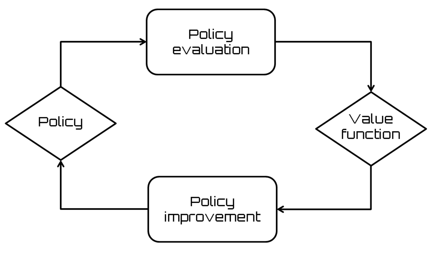
The DP methods approach the resolution of MDP processes through the iteration of two processes called policy evaluation and policy improvement:

• The policy evaluation algorithm consists of applying an iterative method to the resolution of the Bellman equation. Since convergence is guaranteed to us only for k → ∞, we must be content to have good approximations by imposing a stopping condition.
• The policy improvement algorithm improves policy based on current values.

The iteration of the two aforementioned processes is shown in the following diagram:

A disadvantage of the policy iteration algorithm is that we have to evaluate the policy at every step. This involves an iterative process in which we do not know a priori the time of convergence, which will depend, among other things, on how the starting policy was chosen.

One way to overcome this drawback is to cut off the evaluation of the policy at a specific step. This operation does not change the guarantee of convergence to the optimal value. A special case in which the assessment of the policy is blocked step by step (also called sweep) defines the value iteration algorithm. In the value iteration algorithm, a single iteration of calculation of the values is performed between each step of the policy improvement. In the following snippet, a pseudocode for a value-iteration algorithm is shown:

initialize value function V
repeat
   for all s
      for all a
         update Q function
         V = max Q function
until V converge

Thus, in the value iteration algorithm, the system was initiated by setting a random value function. Starting from this value, a new function is sought in an iterative process which, compared to the previous one, has been improved, until reaching the optimal value function.

As we said previously, the DP algorithms are therefore essentially based on two processes that take place in parallel: policy evaluation and policy improvement. The repeated execution of these two processes makes the general process converge toward the optimal solution. In the policy iteration algorithm, the two phases alternate and one ends before the other begins.

In policy iteration algorithms, we start by initializing the system with a random policy, so we first must find the value function of that policy. This phase is called the policy evaluation step. So, we find a new policy, also improved compared to the previous one, based on the previous value function, and so on. In this process, each policy presents an improvement over the previous one until the optimal policy is reached. In the following snippet, a pseudocode for a policy iteration algorithm is shown:

initialize value function V and policy π
repeat
   evaluate V using policy π
   improve π using V
until convergence

DP methods operate through the entire set of states that can be assumed by the environment, performing a complete backup for each state at each iteration. Each update operation performed by the backup updates the value of a state based on the values ​​of all possible successor states, weighed for their probability of occurrence, induced by the policy of choice and by the dynamics of the environment. Full backups are closely related to the Bellman equation; they are nothing more than the transformation of the equation into assignment instructions.

When a complete backup iteration does not bring any change to the state values, convergence is obtained and, therefore, the final state values ​​fully satisfy the Bellman equation. The DP methods are applicable only if there is a perfect model of the environment, which must be equivalent to an MDP.

Precisely for this reason, the DP algorithms are of little use in reinforcement learning, both for their assumption of a perfect model of the environment, and for the high and expensive computation, but it is still opportune to mention them, because they represent the theoretical basis of reinforcement learning. In fact, all the methods of reinforcement learning try to achieve the same goal as that of the DP methods, only with lower computational cost and without the assumption of a perfect model of the environment.

The DP methods converge to the optimal solution with a number of polynomial operations with respect to the number of states n and actions m, against the number of exponential operations m*n required by methods based on direct search.

The DP methods update the estimates of the values of the states, based on the estimates of the values of the successor states, or update the estimates on the basis of past estimates. This represents a special property, which is called bootstrapping. Several methods of reinforcement learning perform bootstrapping, even methods that do not require a perfect model of the environment, as required by the DP methods.

The Monte Carlo (MC) methods for estimating the value function and discovering excellent policies do not require the presence of a model of the environment. They are able to learn through the use of the agent's experience alone or from samples of state sequences, actions, and rewards obtained from the interactions between agent and environment. The experience can be acquired by the agent in line with the learning process or emulated by a previously populated dataset. The possibility of gaining experience during learning (online learning) is interesting because it allows obtaining excellent behavior even in the absence of a priori knowledge of the dynamics of the environment. Even learning through an already populated experience dataset can be interesting, because, if combined with online learning, it makes automatic policy improvement induced by others' experiences possible.

In general, MC methods rely on repeated random sampling to obtain numerical results. To do this, they use randomness to solve deterministic problems. In our case, we will use random sampling of states and action-state pairs and we will look at the rewards and then we will review the policy in an iterative way. The iteration of the process will converge on optimal policy as we explore every possible action-state pair.

For example, we could take the following procedure:

• We will assign a reward of +1 to a right action, -1 to a wrong action, and 0 to a draw.
• We will establish a table in which each key corresponds to a particular state-action pair and each value is the value of that pair. This represents the average reward received for that action in that state.

To solve the reinforcement learning problems, MC methods estimate the value function on the basis of the total sum of rewards, obtained on average in the past episodes. This assumes that the experience is divided into episodes, and that all episodes are composed of a finite number of transitions. This is because, in MC methods, the estimation of new values, and the modification of policies, takes place at the end of each episode. MC methods iteratively estimate policy and value function. In this case, however, each iteration cycle is equivalent to completing an episode—the new estimates of policy and value function occur episode by episode.

The following is a pseudocode for MC policy evaluation:

Initialize
   arbitrary policy π
   arbitrary state-value function
Repeat
   generate episode using π
   for each state s in episode
      the received reinforcement R is added to the set of rewards obtained so far
      estimate the value function on the basis on the average of the total sum of rewards obtained

Usually, the term MC is used for estimation methods, the operations of which involve random components. In this case, the term MC refers to reinforcement learning methods based on total reward averages. Unlike the DP methods that calculate the values ​​for each state, the MC methods calculate the values ​​for each state-action pair, because, in the absence of a model, the only state values ​​are not sufficient to decide which action is best performed in a certain state.

TD learning algorithms are based on reducing the differences between estimates made by the agent at different times. TD algorithms try to predict a quantity that depends on the future values of a given signal. Its name derives from the differences used in predictions on successive time steps to guide the learning process. The prediction at any time is updated to bring it closer to the prediction of the same quantity at the next time step. In reinforcement learning, they are used to predict a measure of the total amount of reward expected in the future.

It is a combination of the ideas of the MC method and the DP.

TD algorithm can learn directly from raw data, without a model of the dynamics of the environment (such as MC). This algorithm updates the estimates based partly on previously learned estimates, without waiting for the final result (bootstrap, like DP). Converge (using a fixed policy) if the time step is sufficiently small, or if it reduces over time.

The consecutive predictions are often related to each other; the TD methods are based on this assumption. These methods try to minimize the error of consecutive time forecasts. To do this, calculate the value function update using the Bellman equation. As already mentioned, to improve the prediction, the bootstrap technique is used, thereby reducing the variance of the prediction in each update step.

The different types of algorithms based on time differences can be distinguished on the basis of the methodology of choosing an action adopted. There are methods of time differences on-policy, in which the update is made on the basis of the results of actions determined by the selected policy and off-policy methods, in which various policies can be assessed through hypothetical actions, not actually undertaken. Unlike on-policy methods, the latter can separate the problem of exploration from that of control, learning tactics not necessarily applied during the learning phase.

The most used TD learning algorithms are the following:

• SARSA
• Q-learning
• Deep Q-learning

In the following sections, we will analyze the main characteristics of the two algorithms and the substantial differences.

The State-action-reward-state-action (SARSA) algorithm implements an on-policy time differences method, in which the update of the action-value function is performed based on the outcome of the transition from state s to state s' through action a, based on a selected policy π (s, a).

There are policies that always choose the action that provides the maximum reward and non-deterministic policies (ε-greedy, ε-soft, softmax), which ensure an element of exploration in the learning phase.

In SARSA, it is necessary to estimate the action-value function q (s, a), because the total value of a state v (s) (value function) is not sufficient in the absence of an environment model to allow the policy to determine, given a state, which action is best performed. In this case, however, the values are estimated step by step following the Bellman equation with the update parameter v (s), considering, however, in place of a state, the state-action pair.

Being of an on-policy nature, SARSA estimates the action-value function based on the behavior of the π policy, and at the same time modifies the greedy behavior of the policy with respect to the updated estimates from the action-value function. The convergence of SARSA, and more generally of all TD methods, depends on the nature of policies.

The following is a pseudocode for the SARSA algorithm:

Initialize
   arbitrary action-value function
Repeat (for each episode)
   Initialize s
   choose a from s using policy from action-value function
   Repeat (for each step in episode)
      take action a
      observe r, s'
      choose a' from s' using policy from action-value function
      update action-value function
      update s,a

The update rule of the action-value function uses all five elements (s_t, a_t, r_{t + 1}, s_{t + 1}, a_{t + 1}); for this reason, it is called SARSA.

Q-learning is one of the most used reinforcement learning algorithms. This is due to its ability to compare the expected utility of the available actions without requiring an environment model. Thanks to this technique, it is possible to find an optimal action for every given state in a finished MDP.

A general solution to the reinforcement learning problem is to estimate, thanks to the learning process, an evaluation function. This function must be able to evaluate, through the sum of the rewards, the optimality/utility or otherwise of a particular policy. In fact, Q-learning tries to maximize the value of the Q function (action-value function), which represents the maximum discounted future reward when we perform actions a in the state s.

Q-learning, like SARSA, estimates the function value q (s, a) incrementally, updating the value of the state-action pair at each step of the environment, following the logic of updating the general formula for estimating the values for the TD methods. Q-learning, unlike SARSA, has off-policy characteristics, that is, while the policy is improved according to the values estimated by q (s, a), the value function updates the estimates following a strictly greedy secondary policy: given a state, the chosen action is always the one that maximizes the value max q (s, a). However, the π policy has an important role in estimating values because, through it, the state-action pairs to be visited and updated are determined.

The following is a pseudocode for a Q-learning algorithm:

Initialize
   arbitrary action-value function
Repeat (for each episode)
   Initialize s
   choose a from s using policy from action-value function
   Repeat (for each step in episode)
      take action a
      observe r, s'
      update action-value function
      update s

Q-learning uses a table to store each state-action pair. At each step, the agent observes the current state of the environment and, using the π policy, selects and executes the action. By executing the action, the agent obtains the reward R_t+1 and the new state S_t+1. At this point the agent is able to calculate Q(S_t, a_t), updating the estimate.

Deep Q-learning represents an evolution of the basic Q-learning method the state-action is replaced by a neural network, with the aim of approximating the optimal value function.

Compared to the previous approaches, where it was used to structure the network in order to request both input and action and providing its expected return, Deep Q-learning revolutionizes the structure in order to request only the state of the environment and supply as many status-action values as there are actions that can be performed in the environment.