
In this section, we will discuss different image manipulation functions (with point transformation and geometric transformation) and how to deal with images of different types. Let us start with that.
An image can be saved in different file formats and in different modes (types). Let us discuss how to handle images of different file formats and types with Python libraries.
Image files can be of different formats. Some of the popular ones include BMP (8-bit, 24-bit, 32-bit), PNG, JPG (JPEG), GIF, PPM, PNM, and TIFF. We do not need to be worried about the specific format of an image file (and how the metadata is stored) to extract data from it. Python image processing libraries will read the image and extract the data, along with some other useful information for us (for example, image size, type/mode, and data type).
Using PIL, we can read an image in one file format and save it to another; for example, from PNG to JPG, as shown in the following:
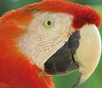
im = Image.open("../images/parrot.png")
print(im.mode)

#  RGB
im.save("../images/parrot.jpg")
But if the PNG file is in the RGBA mode, we need to convert it into the RGB mode before we save it as JPG, as otherwise it will give an error. The next code block shows how to first convert and then save:
im = Image.open("../images/hill.png")
print(im.mode)
# RGBA
im.convert('RGB').save("../images/hill.jpg") # first convert to RGB modeAn image can be of the following different types:
- Single channel images—each pixel is represented by a single value:
- Binary (monochrome) images (each pixel is represented by a single 0-1 bit)
- Gray-level images (each pixel can be represented with 8-bits and can have values typically in the range of 0-255)
- Multi-channel images—each pixel is represented by a tuple of values:
- 3-channel images; for example, the following:
- RGB images—each pixel is represented by three-tuple (r, g, b) values, representing red, green, and blue channel color values for every pixel.
- HSV images—each pixel is represented by three-tuple (h, s, v) values, representing hue (color), saturation (colorfulness—how much the color is mixed with white), and value (brightness—how much the color is mixed with black) channel color values for every pixel. The HSV model describes colors in a similar manner to how the human eye tends to perceive colors.
- Four-channel images; for example, RGBA images—each pixel is represented by three-tuple (r, g, b, α) values, the last channel representing the transparency.
- 3-channel images; for example, the following:
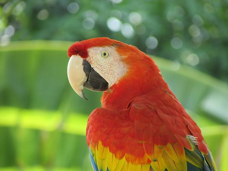
We can convert an RGB image into a grayscale image while reading the image itself. The following code does exactly that:
im = imread("images/parrot.png", as_gray=True)
print(im.shape)
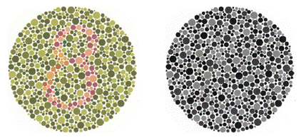
#(362L, 486L)Note that we can lose some information while converting into grayscale for some colored images. The following code shows such an example with Ishihara plates, used to detect color-blindness. This time, the rgb2gray()function is used from the color module, and both the color and the grayscale images are shown side by side. As can be seen in the following figure, the number 8 is almost invisible in the grayscale version:
im = imread("../images/Ishihara.png")
im_g = color.rgb2gray(im)
plt.subplot(121), plt.imshow(im, cmap='gray'), plt.axis('off')
plt.subplot(122), plt.imshow(im_g, cmap='gray'), plt.axis('off')
plt.show()
The next figure shows the output of the previous code—the colored image and the grayscale image obtained from it:
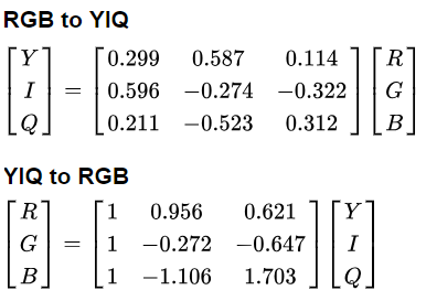
The following represents a few popular channels/color spaces for an image: RGB, HSV, XYZ, YUV, YIQ, YPbPr, YCbCr, and YDbDr. We can use Affine mappings to go from one color space to another. The following matrix represents the linear mapping from the RGB to YIQ color space:
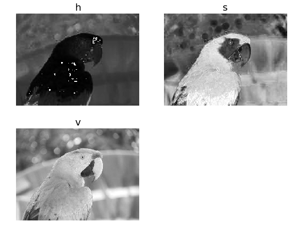
We can convert from one color space into another using library functions; for example, the following code converts an RGB color space into an HSV color space image:
im = imread("../images/parrot.png")
im_hsv = color.rgb2hsv(im)
plt.gray()
plt.figure(figsize=(10,8))
plt.subplot(221), plt.imshow(im_hsv[...,0]), plt.title('h', size=20), plt.axis('off')
plt.subplot(222), plt.imshow(im_hsv[...,1]), plt.title('s', size=20), plt.axis('off')
plt.subplot(223), plt.imshow(im_hsv[...,2]), plt.title('v', size=20), plt.axis('off')
plt.subplot(224), plt.axis('off')
plt.show()
The next figure shows the h (heu or color: dominant wave length of reflected light), s (saturation or chroma) and v (value or brightness/luminescence) channels of the parrot HSV image, created using the previous code:
Similarly, we can convert the image into the YUV color space using the rgb2yuv() function.
As we have already discussed, PIL uses the Image object to store an image, whereas scikit-image uses the numpy ndarray data structure to store the image data. The next section describes how to convert between these two data structures.
The following code block shows how to convert from the PIL Image object into numpy ndarray (to be consumed by scikit-image):
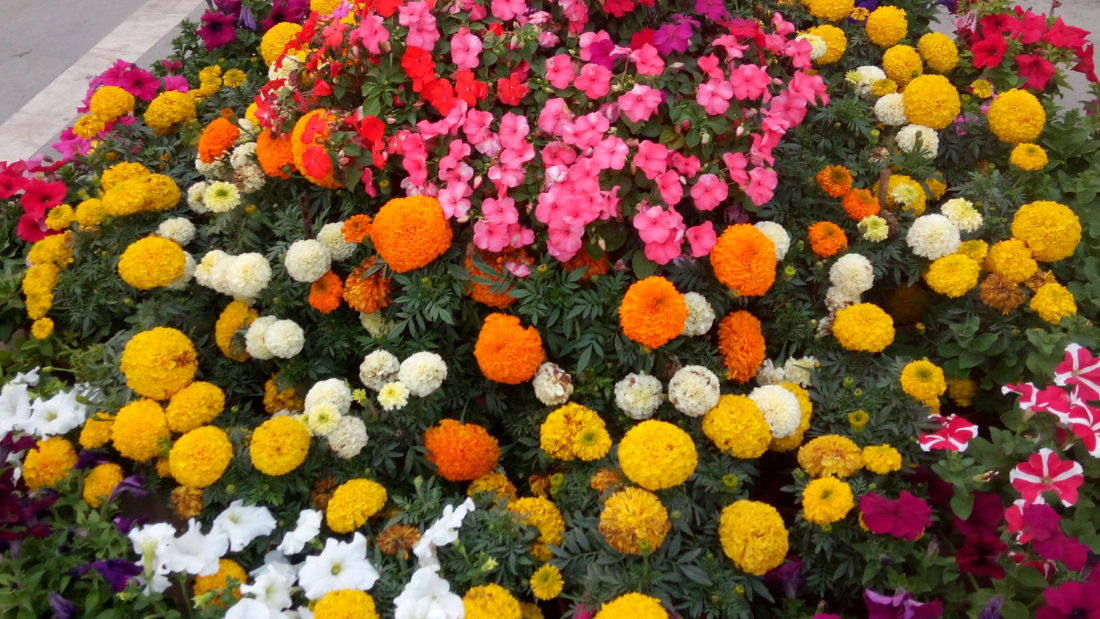
im = Image.open('../images/flowers.png') # read image into an Image object with PIL
im = np.array(im) # create a numpy ndarray from the Image object
imshow(im) # use skimage imshow to display the image
plt.axis('off'), show()
The next figure shows the output of the previous code, which is an image of flowers:
The following code block shows how to convert from numpy ndarray into a PIL Image object. When run, the code shows the same output as the previous figure:
im = imread('../images/flowers.png') # read image into numpy ndarray with skimage
im = Image.fromarray(im) # create a PIL Image object from the numpy ndarray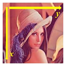
im.show() # display the image with PIL Image.show() methodDifferent Python libraries can be used for basic image manipulation. Almost all of the libraries store an image in numpy ndarray (a 2-D array for grayscale and a 3-D array for an RGB image, for example). The following figure shows the positive x and y directions (the origin being the top-left corner of the image 2-D array) for the colored lena image:
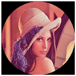
The next code block shows how slicing and masking with numpy arrays can be used to create a circular mask on the lena image:
lena = mpimg.imread("../images/lena.jpg") # read the image from disk as a numpy ndarray
print(lena[0, 40])
# [180  76  83]
# print(lena[10:13, 20:23,0:1]) # slicing
lx, ly, _ = lena.shape
X, Y = np.ogrid[0:lx, 0:ly]
mask = (X - lx / 2) ** 2 + (Y - ly / 2) ** 2 > lx * ly / 4
lena[mask,:] = 0 # masks
plt.figure(figsize=(10,10))
plt.imshow(lena), plt.axis('off'), plt.show()
The following figure shows the output of the code:
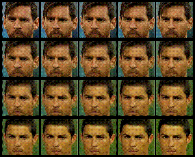
The following code block shows how to start from one face image (image1 being the face of Messi) and end up with another image (image2 being the face of Ronaldo) by using a linear combination of the two image numpy ndarrays given with the following equation:

We do this by iteratively increasing α from 0 to 1:
im1 = mpimg.imread("../images/messi.jpg") / 255 # scale RGB values in [0,1]
im2 = mpimg.imread("../images/ronaldo.jpg") / 255
i = 1
plt.figure(figsize=(18,15))
for alpha in np.linspace(0,1,20):
 plt.subplot(4,5,i)
 plt.imshow((1-alpha)*im1 + alpha*im2)
 plt.axis('off')
 i += 1
plt.subplots_adjust(wspace=0.05, hspace=0.05)
plt.show()
The next figure shows the sequence of the α-blended images created using the previous code by cross-dissolving Messi's face image into Ronaldo's. As can be seen from the sequence of intermediate images in the figure, the face morphing with simple blending is not very smooth. In upcoming chapters, we shall see more advanced techniques for image morphing:
PIL provides us with many functions to manipulate an image; for example, using a point transformation to change pixel values or to perform geometric transformations on an image. Let us first start by loading the parrot PNG image, as shown in the following code:
im = Image.open("../images/parrot.png")        # open the image, provide the correct path
print(im.width, im.height, im.mode, im.format) # print image size, mode and format
# 486 362 RGB PNG
The next few sections describe how to do different types of image manipulations with PIL.
We can use the crop() function with the desired rectangle argument to crop the corresponding area from the image, as shown in the following code:
im_c = im.crop((175,75,320,200)) # crop the rectangle given by (left, top, right, bottom) from the image
im_c.show()
The next figure shows the cropped image created using the previous code:
In order to increase or decrease the size of an image, we can use the resize() function, which internally up-samples or down-samples the image, respectively. This will be discussed in detail in the next chapter.
Resizing to a larger image
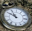
Let us start with a small clock image of a size of 149 x 97 and create a larger size image. The following code snippet shows the small clock image we will start with:
im = Image.open("../images/clock.jpg")
print(im.width, im.height)
# 107 105
im.show()
The output of the previous code, the small clock image, is shown as follows:
The next line of code shows how the resize() function can be used to enlarge the previous input clock image (by a factor of 5) to obtain an output image of a size 25 times larger than the input image by using bi-linear interpolation (an up-sampling technique). The details about how this technique works will be described in the next chapter:
im_large = im.resize((im.width*5, im.height*5), Image.BILINEAR) # bi-linear interpolation
Resizing to a smaller image
Now let us do the reverse: start with a large image of the Victoria Memorial Hall (of a size of 720 x 540) and create a smaller-sized image. The next code snippet shows the large image to start with:
im = Image.open("../images/victoria_memorial.png")
print(im.width, im.height)
# 720 540
im.show()
The output of the previous code, the large image of the Victoria Memorial Hall, is shown as follows:
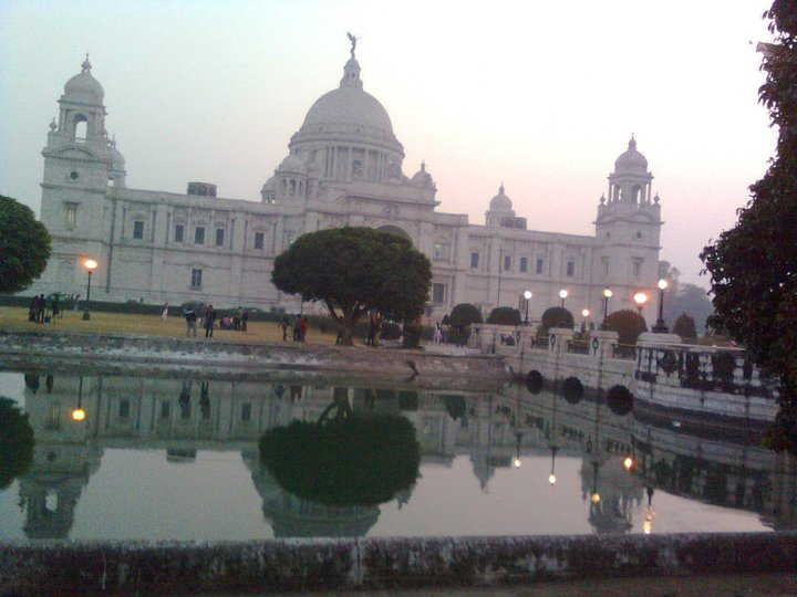
The next line of code shows how the resize() function can be used to shrink the previous image of the Victoria Memorial Hall (by a factor of 5) to resize it to an output image of a size 25 times smaller than the input image by using anti-aliasing (a high-quality down-sampling technique). We will see how it works in the next chapter:
im_small = im.resize((im.width//5, im.height//5), Image.ANTIALIAS)
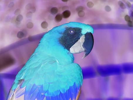
We can use the point() function to transform each pixel value with a single-argument function. We can use it to negate an image, as shown in the next code block. The pixel values are represented using 1-byte unsigned integers, which is why subtracting it from the maximum possible value will be the exact point operation required on each pixel to get the inverted image:
im = Image.open("../images/parrot.png")
im_t = im.point(lambda x: 255 - x)
im_t.show()
The next figure shows the negative image, the output of the previous code:
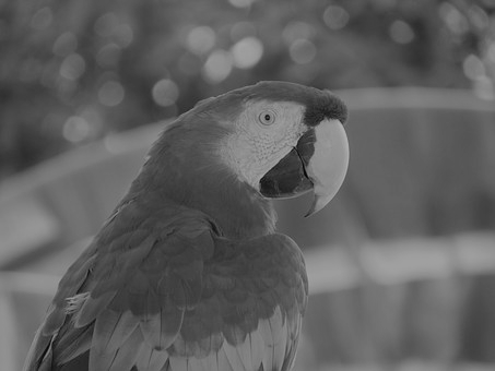
We can use the convert() function with the 'L' parameter to change an RGB color image into a gray-level image, as shown in the following code:
im_g = im.convert('L') # convert the RGB color image to a grayscale imageWe are going to use this image for the next few gray-level transformations.
Here we explore a couple of transformations where, using a function, each single pixel value from the input image is transferred to a corresponding pixel value for the output image. The function point() can be used for this. Each pixel has a value in between 0 and 255, inclusive.
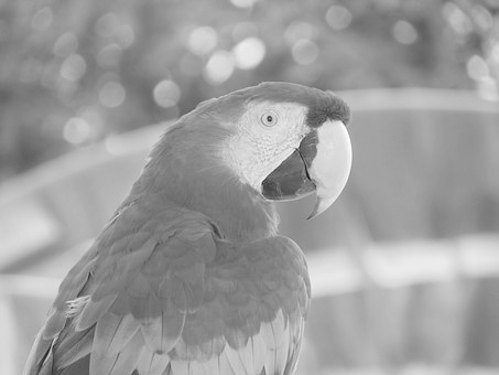
Log transformation
The log transformation can be used to effectively compress an image that has a dynamic range of pixel values. The following code uses the point transformation for logarithmic transformation. As can be seen, the range of pixel values is narrowed, the brighter pixels from the input image have become darker, and the darker pixels have become brighter, thereby shrinking the range of values of the pixels:
im_g.point(lambda x: 255*np.log(1+x/255)).show()
The next figure shows the output log-transformed image produced by running the previous line of code:
Power-law transformation
This transformation is used as γ correction for an image. The next line of code shows how to use the point() function for a power-law transformation, where γ = 0.6:
im_g.point(lambda x: 255*(x/255)**0.6).show()
The next figure shows the output power-law-transformed image produced by running the preceding line of code:
In this section, we will discuss another set of transformations that are done by multiplying appropriate matrices (often expressed in homogeneous coordinates) with the image matrix. These transformations change the geometric orientation of an image, hence the name.
Reflecting an image
We can use the transpose() function to reflect an image with regard to the horizontal or vertical axis:
im.transpose(Image.FLIP_LEFT_RIGHT).show() # reflect about the vertical axis
The next figure shows the output image produced by running the previous line of code:
Rotating an image
We can use the rotate() function to rotate an image by an angle (in degrees):
im_45 = im.rotate(45) # rotate the image by 45 degrees
im_45.show()          # show the rotated image
The next figure shows the rotated output image produced by running the preceding line of code:
Applying an Affine transformation on an image
A 2-D Affine transformation matrix, T, can be applied on each pixel of an image (in homogeneous coordinates) to undergo an Affine transformation, which is often implemented with inverse mapping (warping). An interested reader is advised to refer to this article (https://sandipanweb.wordpress.com/2018/01/21/recursive-graphics-bilinear-interpolation-and-image-transformation-in-python/) to understand how these transformations can be implemented (from scratch).
The following code shows the output image obtained when the input image is transformed with a shear transform matrix. The data argument in the transform() function is a 6-tuple (a, b, c, d, e, f), which contains the first two rows from an Affine transform matrix. For each pixel (x, y) in the output image, the new value is taken from a position (a x + b y + c, d x + e y + f) in the input image, which is rounded to nearest pixel. The transform() function can be used to scale, translate, rotate, and shear the original image:
im = Image.open("../images/parrot.png")
im.transform((int(1.4*im.width), im.height), Image.AFFINE, data=(1,-0.5,0,0,1,0)).show() # shear
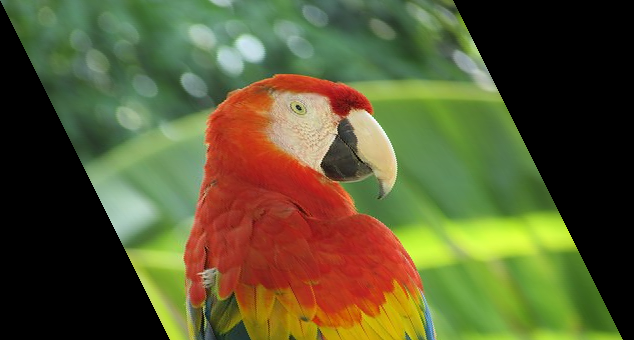
The next figure shows the output image with shear transform, produced by running the previous code:
Perspective transformation
We can run a perspective transformation on an image with the transform() function by using the Image.PERSPECTIVE argument, as shown in the next code block:
params = [1, 0.1, 0, -0.1, 0.5, 0, -0.005, -0.001]
im1 = im.transform((im.width//3, im.height), Image.PERSPECTIVE, params, Image.BICUBIC)
im1.show()
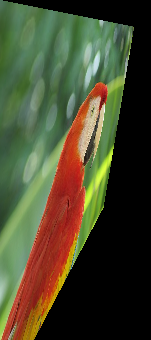
The next figure shows the image obtained after the perspective projection, by running the preceding code block:
We can use the putpixel() function to change a pixel value in an image. Next, let us discuss a popular application of adding noise to an image using the function.
Adding salt and pepper noise to an image
We can add some salt-and-pepper noise to an image by selecting a few pixels from the image randomly and then setting about half of those pixel values to black and the other half to white. The next code snippet shows how to add the noise:
# choose 5000 random locations inside image
im1 = im.copy() # keep the original image, create a copy
n = 5000
x, y = np.random.randint(0, im.width, n), np.random.randint(0, im.height, n)
for (x,y) in zip(x,y):
 im1.putpixel((x, y), ((0,0,0) if np.random.rand() < 0.5 else (255,255,255))) # salt-and-pepper noise
im1.show()
The following figure shows the output noisy image generated by running the previous code:
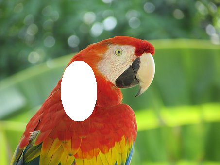
We can draw lines or other geometric shapes on an image (for example, the ellipse() function to draw an ellipse) from the PIL.ImageDraw module, as shown in the next Python code snippet:
im = Image.open("../images/parrot.png")
draw = ImageDraw.Draw(im)
draw.ellipse((125, 125, 200, 250), fill=(255,255,255,128))
del draw
im.show()
The following figure shows the output image generated by running the previous code:
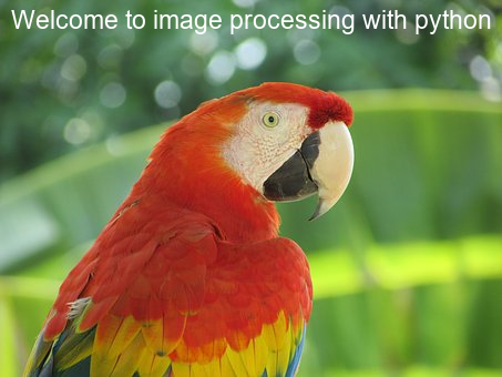
We can add text to an image using the text() function from the PIL.ImageDraw module, as shown in the next Python code snippet:
draw = ImageDraw.Draw(im)
font = ImageFont.truetype("arial.ttf", 23) # use a truetype font
draw.text((10, 5), "Welcome to image processing with python", font=font)
del draw
im.show()
The following figure shows the output image generated by running the previous code:
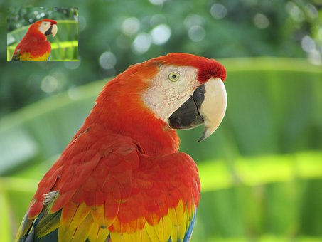
We can create a thumbnail from an image with the thumbnail() function, as shown in the following:
im_thumbnail = im.copy() # need to copy the original image first
im_thumbnail.thumbnail((100,100))
# now paste the thumbnail on the image
im.paste(im_thumbnail,(10,10))im.save("../images/parrot_thumb.jpg")im.show()
The figure shows the output image generated by running the preceding code snippet:
We can use the stat module to compute the basic statistics (mean, median, standard deviation of pixel values of different channels, and so on) of an image, as shown in the following:
s = stat.Stat(im)
print(s.extrema) # maximum and minimum pixel values for each channel R, G, B
# [(4, 255), (0, 255), (0, 253)]
print(s.count)
# [154020, 154020, 154020]
print(s.mean)
# [125.41305674587716, 124.43517724970783, 68.38463186599142]
print(s.median)
# [117, 128, 63]
print(s.stddev)
# [47.56564506512579, 51.08397900881395, 39.067418896260094]
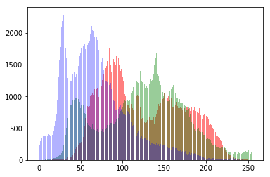
The histogram() function can be used to compute the histogram (a table of pixel values versus frequencies) of pixels for each channel and return the concatenated output (for example, for an RGB image, the output contains 3 x 256 = 768 values):
pl = im.histogram()
plt.bar(range(256), pl[:256], color='r', alpha=0.5)
plt.bar(range(256), pl[256:2*256], color='g', alpha=0.4)
plt.bar(range(256), pl[2*256:], color='b', alpha=0.3)
plt.show()
The following figure shows the R, G, and B color histograms plotted by running the previous code:
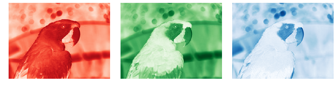
We can use the split() function to separate the channels of a multi-channel image, as is shown in the following code for an RGB image:
ch_r, ch_g, ch_b = im.split() # split the RGB image into 3 channels: R, G and B
# we shall use matplotlib to display the channels
plt.figure(figsize=(18,6))
plt.subplot(1,3,1); plt.imshow(ch_r, cmap=plt.cm.Reds); plt.axis('off')
plt.subplot(1,3,2); plt.imshow(ch_g, cmap=plt.cm.Greens); plt.axis('off')
plt.subplot(1,3,3); plt.imshow(ch_b, cmap=plt.cm.Blues); plt.axis('off')
plt.tight_layout()
plt.show() # show the R, G, B channels
The following figure shows three output images created for each of the R (red), G (green), and B (blue) channels generated by running the previous code:
We can use themerge()function to combine the channels of a multi-channel image, as is shown in the following code, wherein the color channels obtained by splitting the parrot RGB image are merged after swapping the red and blue channels:
im = Image.merge('RGB', (ch_b, ch_g, ch_r)) # swap the red and blue channels obtained last time with split()
im.show()
The following figure shows the RGB output image created by merging the B, G, and R channels by running the preceding code snippet:
The blend() function can be used to create a new image by interpolating two given images (of the same size) using a constant, α. Both images must have the same size and mode. The output image is given by the following:
out = image1 * (1.0 - α) + image2 * α
If α is 0.0, a copy of the first image is returned. If α is 1.0, a copy of the second image is returned. The next code snippet shows an example:
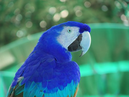
im1 = Image.open("../images/parrot.png")
im2 = Image.open("../images/hill.png")
# 453 340 1280 960 RGB RGBA
im1 = im1.convert('RGBA') # two images have different modes, must be converted to the same mode
im2 = im2.resize((im1.width, im1.height), Image.BILINEAR) # two images have different sizes, must be converted to the same size
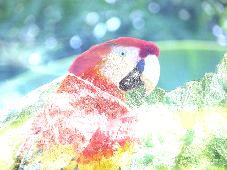
im = Image.blend(im1, im2, alpha=0.5).show()The following figure shows the output image generated by blending the previous two images:
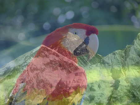
An image can be superimposed on top of another by multiplying two input images (of the same size) pixel by pixel. The next code snippet shows an example:
im1 = Image.open("../images/parrot.png")
im2 = Image.open("../images/hill.png").convert('RGB').resize((im1.width, im1.height))
multiply(im1, im2).show()
The next figure shows the output image generated when superimposing two images by running the preceding code snippet:
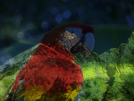
The next code snippet shows how an image can be generated by adding two input images (of the same size) pixel by pixel:
add(im1, im2).show()
The next figure shows the output image generated by running the previous code snippet:
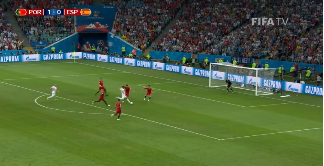
The following code returns the absolute value of the pixel-by-pixel difference between images. Image difference can be used to detect changes between two images. For example, the next code block shows how to compute the difference image from two successive frames from a video recording (from YouTube) of a match from the 2018 FIFA World Cup:
from PIL.ImageChops import subtract, multiply, screen, difference, add
im1 = Image.open("../images/goal1.png") # load two consecutive frame images from the video
im2 = Image.open("../images/goal2.png")
im = difference(im1, im2)
im.save("../images/goal_diff.png")
plt.subplot(311)
plt.imshow(im1)
plt.axis('off')
plt.subplot(312)
plt.imshow(im2)
plt.axis('off')
plt.subplot(313)
plt.imshow(im), plt.axis('off')
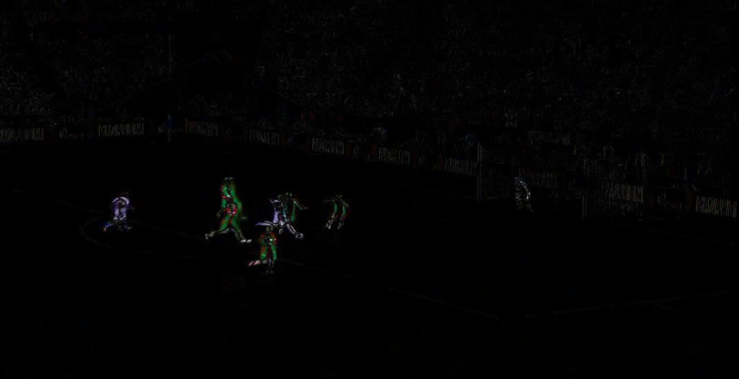
plt.show()The next figure shows the output of the code, with the consecutive frame images followed by their difference image:
First frame

Second frame
The difference image
The subtract() function can be used to first subtract two images, followed by dividing the result by scale (defaults to 1.0) and adding the offset (defaults to 0.0). Similarly, the screen() function can be used to superimpose two inverted images on top of each other.
As done previously using the PIL library, we can also use the scikit-image library functions for image manipulation. Some examples are shown in the following sections.
The scikit-image transform module's warp() function can be used for inverse warping for the geometric transformation of an image (discussed in a previous section), as demonstrated in the following examples.
Applying an Affine transformation on an image
We can use the SimilarityTransform() function to compute the transformation matrix, followed by warp() function, to carry out the transformation, as shown in the next code block:
im = imread("../images/parrot.png")
tform = SimilarityTransform(scale=0.9, rotation=np.pi/4,translation=(im.shape[0]/2, -100))
warped = warp(im, tform)
import matplotlib.pyplot as plt
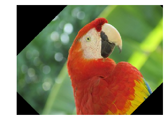
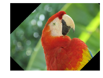
plt.imshow(warped), plt.axis('off'), plt.show()The following figure shows the output image generated by running the previous code snippet:
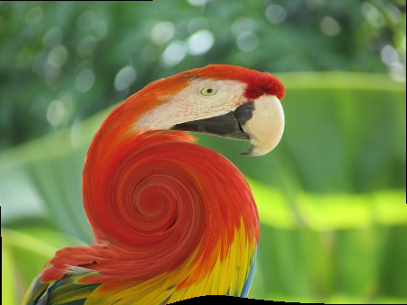
This is a non-linear transform defined in the scikit-image documentation. The next code snippet shows how to use the swirl()function to implement the transform, where strength is a parameter to the function for the amount of swirl, radius indicates the swirl extent in pixels, and rotation adds a rotation angle. The transformation of radius into r is to ensure that the transformation decays to ≈ 1/1000th ≈ 1/1000th within the specified radius:
im = imread("../images/parrot.png")
swirled = swirl(im, rotation=0, strength=15, radius=200)
plt.imshow(swirled)
plt.axis('off')
plt.show()
The next figure shows the output image generated with swirl transformation by running the previous code snippet:
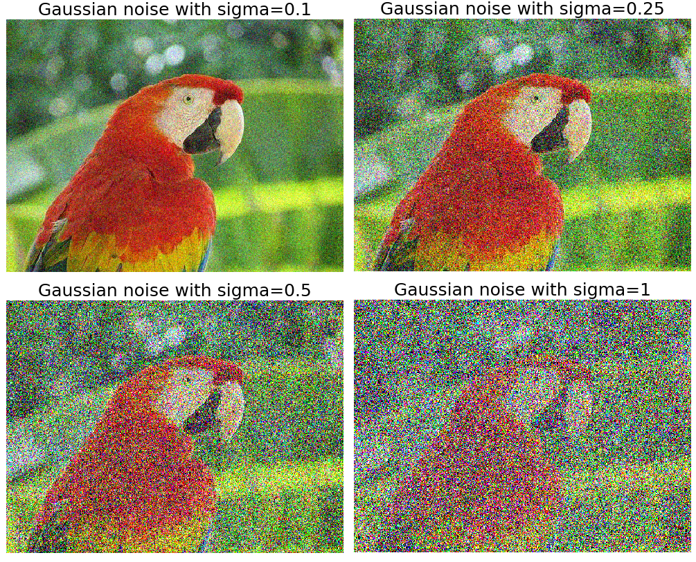
We can use the random_noise() function to add different types of noise to an image. The next code example shows how Gaussian noise with different variances can be added to an image:
im = img_as_float(imread("../images/parrot.png"))
plt.figure(figsize=(15,12))
sigmas = [0.1, 0.25, 0.5, 1]
for i in range(4):
noisy = random_noise(im, var=sigmas[i]**2)
plt.subplot(2,2,i+1)
plt.imshow(noisy)
plt.axis('off')
plt.title('Gaussian noise with sigma=' + str(sigmas[i]), size=20)
plt.tight_layout()
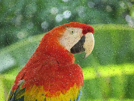
plt.show()The next figure shows the output image generated by adding Gaussian noises with different variance by running the previous code snippet. As can be seen, the more the standard deviation of the Gaussian noise, the noisier the output image:
We can compute the cumulative distribution function (CDF) for a given image with the cumulative_distribution() function, as we shall see in the image enhancement chapter. For now, the reader is encouraged to find the usage of this function to compute the CDF.
We can use the pylab module from the matplotlib library for image manipulation. The next section shows an example.
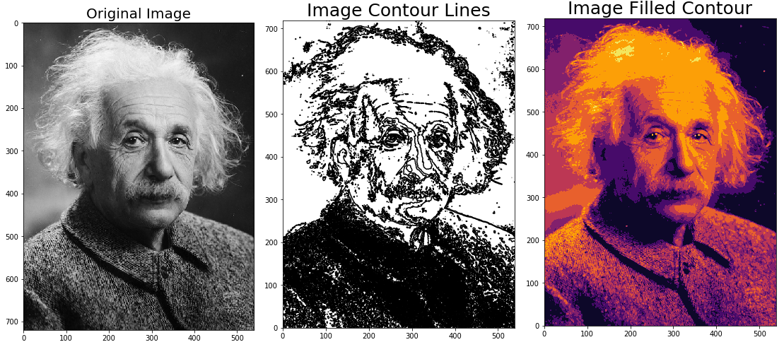
A contour line for an image is a curve connecting all of the pixels where they have the same particular value. The following code block shows how to draw the contour lines and filled contours for a grayscale image of Einstein:
im = rgb2gray(imread("../images/einstein.jpg")) # read the image from disk as a numpy ndarray
plt.figure(figsize=(20,8))
plt.subplot(131), plt.imshow(im, cmap='gray'), plt.title('Original Image', size=20)
plt.subplot(132), plt.contour(np.flipud(im), colors='k', levels=np.logspace(-15, 15, 100))
plt.title('Image Contour Lines', size=20)
plt.subplot(133), plt.title('Image Filled Contour', size=20), plt.contourf(np.flipud(im), cmap='inferno')
plt.show()
The next figure shows the output of the previous code: