Data is everywhere. At this very moment, thousands of systems are collecting records that make up the history of specific services, together with logs, user interactions, and many other context-dependent elements. Only a decade ago, most companies couldn't even manage 1% of their data efficiently. For this reason, databases were periodically pruned and only important data used to be retained in permanent storage servers.

Conversely, nowadays almost every company can exploit cloud infrastructures that scale in order to cope with the increasing volume of incoming data. Tools such as Apache Hadoop or Apache Spark allow both data scientists and engineers to implement complex pipelines involving extremely large volumes of data. At this point, all the barriers have been torn down and a democratized process is in place. However, what is the actual value of these large datasets? From a business viewpoint, the information is valuable only when it can help make the right decisions, reducing uncertainty and providing better contextual insight. This means that, without the right tools and knowledge, a bunch of data is only a cost to the company that needs to be limited to increase the margins.

Machine learning is a large branch of computer science (in particular, artificial intelligence), which aims to implement descriptive and predictive models of reality by exploiting existing datasets. As this book is dedicated to practical unsupervised solutions, we are going to focus only on algorithms that describe the context by looking for hidden causes and relationships. However, even if only from a theoretical viewpoint, it's helpful to show the main differences between machine learning problems. Only complete awareness (not limited to mere technical aspects) of the goals can lead to a rational answer to the initial question, Why do we need machine learning?

We can start by saying that human beings have extraordinary cognitive abilities, which have inspired many systems, but they lack analytical skills when the number of elements increases significantly. For example, if you're a teacher who is meeting his/her class for the first time, you'll be able to compute a rough estimate of the percentage of female students after taking a glance at the entire group. Usually, the estimate is likely to be accurate and close to the actual count, even if the estimation is made by two or more individuals. However, if we repeat the experiment with the entire population of a school gathered in a courtyard, the distinction of gender will not be evident. This is because all students are clearly visible in the class; however, telling the sexes apart in the courtyard is limited by certain factors (for example, taller people can hide shorter ones). Getting rid of the analogy, we can say that a large amount of data usually carries a lot of information. In order to extract and categorize the information, it's necessary to take an automated approach.

Before moving to the next section, let's discuss the concepts of descriptive, diagnostic, predictive, and prescriptive analyses, originally defined by Gartner. However, in this case, we want to focus on a system (for example, a generic context) that we are analyzing in order to gain more and more control over its behavior.

The complete process is represented in the following diagram:

The first problem to solve in almost any data science scenario concerns understanding its nature. We need to know how the system works or what a dataset is describing. Without this analysis, our knowledge is too limited to make any assumption or hypothesis. For example, we can observe a chart of the average temperature in a city for several years. If we are unable to describe the time series discovering the correlation, seasonalities, and trends, any other question remains unsolved. In our specific context, if we don't discover the similarities between groups of objects, we cannot try to find out a way to summarize their common features. The data scientist has to employ specific tools for every particular problem, but, at the end of this stage, all possible (and helpful) questions must be answered.

Moreover, as this process must have clear business value, it's important to involve different stakeholders with the purpose of gathering their knowledge and converting it into a common language. For example, when working with healthcare data, a physician might talk about hereditary factors, but for our purpose, it's preferable to say that there's a correlation among some samples, so we're not fully authorized to treat them as statistically independent elements. In general, the outcome of descriptive analysis is a summary containing all metric evaluations and conclusions that are necessary to qualify the context, and reducing uncertainty. In the example of the temperature chart, the data scientist should be able to answer the auto-correlation, the periodicity of the peaks, the number of potential outliers, and the presence of trends.

Till now, we have worked with output data, which has been observed after a specific underlying process has generated it. The natural question after having described the system relates to the causes. Temperature depends on many meteorological and geographical factors, which can be either easily observable or completely hidden. Seasonality in the time series is clearly influenced by the period of the year, but what about the outliers?

For example, we have discovered a peak in a region identified as winter. How can we justify it? In a simplistic approach, this can be considered as a noisy outlier that can be filtered out. However, if it has been observed and there's a ground truth behind the measure (for example, all the parties agree that it's not an error), we should assume the presence of a hidden (or latent) cause.

It can be surprising, but the majority of more complex scenarios are characterized by a huge number of latent causes (sometimes called factors) that are too difficult to analyze. In general, this is not a bad condition but, as we're going to discuss, it's important to include them in the model to learn their influence through the dataset.

On the other hand, deciding to drop all unknown elements means reducing the predictive ability of the model with a proportional loss of accuracy. Therefore, the primary goal of diagnostic analysis is not necessarily to find out all the causes but to list the observable and measurable elements (known as factors), together with all the potential latent ones (which are generally summarized into a single global element).

To a certain extent, a diagnostic analysis is often similar to a reverse-engineering process, because we can easily monitor the effects, but it's more difficult to detect existing relationships between potential causes and observable effects. For this reason, such an analysis is often probabilistic and helps find the probability that a certain identified cause brings about a specific effect. In this way, it's also easier to exclude non-influencing elements and to determine relationships that were initially excluded. However, this process requires a deeper knowledge of statistical learning methods and it won't be discussed in this book, apart from a few examples, such as a Gaussian mixture.

Once the overall descriptive knowledge has been gathered and the awareness about the underlying causes is satisfactory, it's possible to create predictive models. The goal of these models is to infer future outcomes according to the history and the structure of the model itself. In many cases, this phase is analyzed together with the next one because we are seldom interested in a free evolution of the system (for example, how the temperature will change in the next month), but rather in the ways we can influence the output.

That said, let's focus only on the predictions, considering the most important elements that should be taken into account. The first consideration is about the nature of the processes. We don't need machine learning for deterministic processes unless their complexity is so high that we're forced to consider them as black boxes. The vast majority of examples we are going to discuss are about stochastic processes where the uncertainty cannot be removed. For example, we know that the temperature in a day can be modeled as a conditional probability (for example, a Gaussian) dependent on the previous observations. Therefore, a prediction sets out not to turn the system into a deterministic one, which is impossible, but to reduce the variance of the distribution, so that the probability is high only for a short range of temperatures. On the other hand, as we know that many latent factors work behind the scene, we can never accept a model based on spiky distributions (for example, on a single outcome with probability 1) because this choice would have a terribly negative impact on the final accuracy.

If our model is parameterized with variables subject to the learning process (for example, the means and covariance matrices of the Gaussians), our goal is to find out the optimal balance in the so-called bias-variance trade-off. As this chapter is an introductory one, we are not formalizing the concepts with mathematical formulas, but we need a practical definition (further details can be found in Bonaccorso G., Mastering Machine Learning Algorithms, Packt, 2018).

The common term to define a statistical predictive model is an estimator. Hence the bias of an estimator is the measurable effect of incorrect assumptions and learning procedures. In other words, if the mean of a process is 5.0 and our estimations have a mean of 3.0, we can say the model is biased. Considering the previous example, we are working with a biased estimator if the expected value of the error between the observed value and the prediction is not null. It's important to understand that we are not saying that every single estimation must have a null error, but while collecting enough samples and computing the mean, its value should be very close to zero (it can be zero only with infinite samples). Whenever it is rather larger than zero, it means that our model is not able to predict training values correctly. It's obvious that we are looking for unbiased estimators that, on average, yield accurate predictions.

On the other hand, the variance of an estimator is a measure of the robustness in the presence of samples not belonging to the training set. At the beginning of this section, we said that our processes are normally stochastic. This means that any dataset must be considered as drawn from a specific data-generating process p_data. If we have enough representative elements x_i ∈ X, we can suppose that training a classifier using the limited dataset X leads to a model that is able to classify all potential samples that can be drawn from p_data.

For example, if we need to model a face classifier whose context is limited to portraits (no further face poses are allowed), we can collect a number of portraits of different individuals. Our only concern is not to exclude categories that can be present in real life. Let's assume that we have 10,000 images of individuals of different ages and genders, but we don't have any portraits with a hat. When the system is in production, we receive a call from our customer saying that the system misclassifies many pictures. After analysis, we discover that they always represent people wearing hats. It's clear that our model is not responsible for the error because it has been trained with samples representing only a region of the data generating process. Therefore, in order to solve the problem, we collect other samples and we repeat the training process. However, now we decide to use a more complex model, expecting that it will work better. Unfortunately, we observe a worse validation accuracy (for example, the accuracy on a subset that is not used in the training phase), together with a higher training accuracy. What happened here?

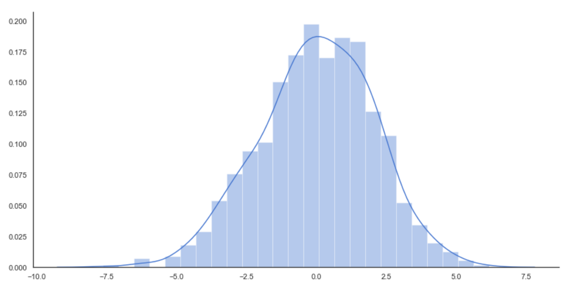
When an estimator learns to classify the training set perfectly but its ability on never-seen samples is poor, we say that it is overfitted and its variance is too high for the specific task (conversely, an underfitted model has a large bias and all predictions are very inaccurate). Intuitively, the model has learned too much about the training data and it has lost the ability to generalize. To better understand this concept, let's look at a Gaussian data generating process, as shown in the following graph:

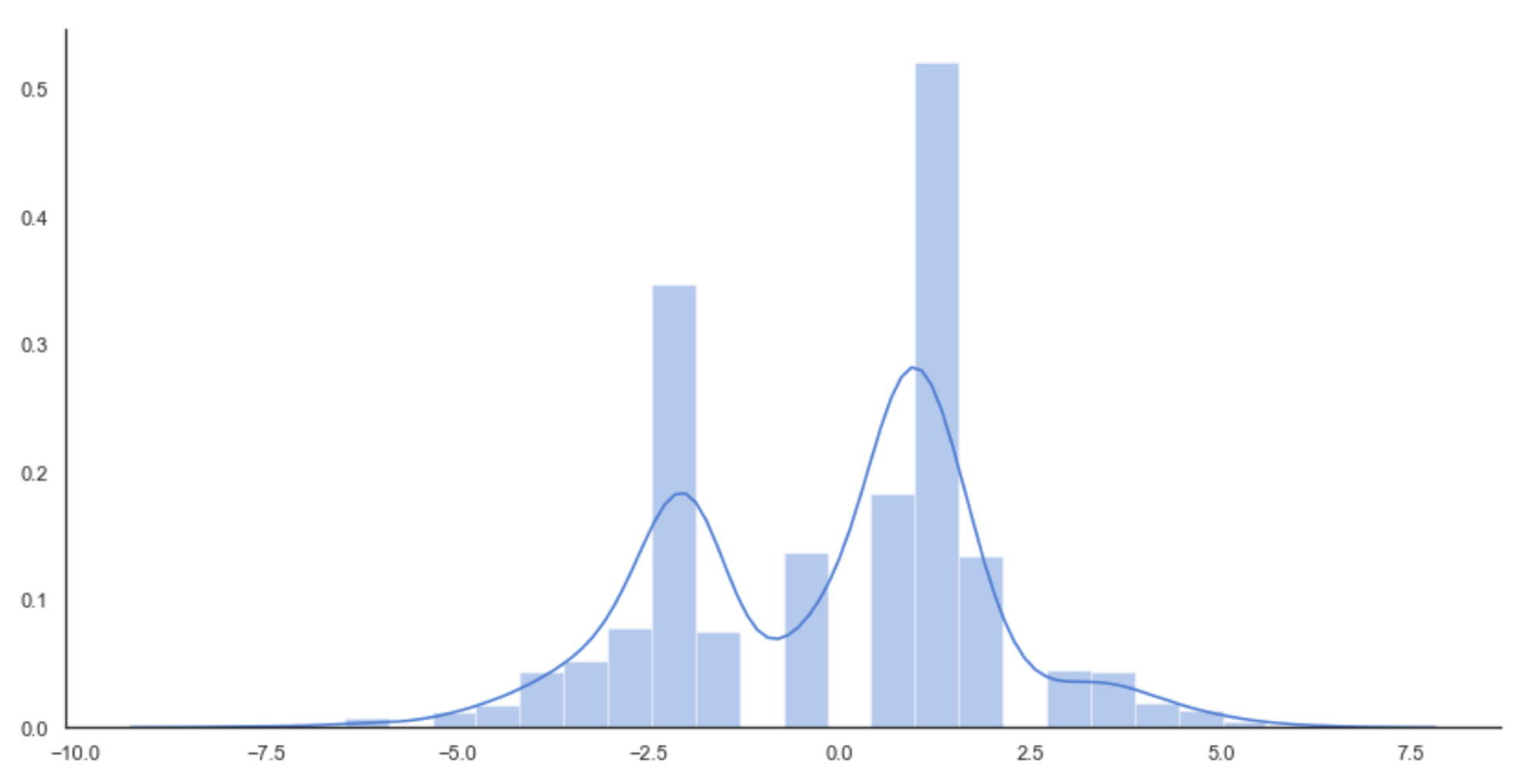
If the training set hasn't been sampled in a perfectly uniform way or it's partially unbalanced (some classes have fewer samples than the other ones), or if the model is prone to overfitting, the result can be represented by an inaccurate distribution, as follows:

In this case, the model has been forced to learn the details of the training set until it has excluded many potential samples from the distribution. The result is no more Gaussian, but a double-peaked distribution, where some probabilities are erroneously low. Of course, the test and validation sets are sampled from the small regions not covered by the training set (as there's no overlap between training data and validation data), therefore the model will fail in its task providing completely incorrect results.

In other words, we can say that the variance is too high because the model has learned to work with too many details, increasing the range of possibilities of different classifications over a reasonable threshold. For example, the portrait classifier could have learned that people with blue glasses are always male in the age range 30–40 (this is an unrealistic situation because the detail level is generally very low, however, it's helpful to understand the nature of the problem).

We can summarize by saying that a good predictive model must have very low bias and proportionally low variance. Unfortunately, it's generally impossible to minimize both measures effectively, so a trade-off must be accepted.

A system with a good generalization ability will be likely to have a higher bias because it is unable to capture all the details. Conversely, a high variance allows a very small bias, but the ability of the model is almost limited to the training set. In this book, we are not going to talk about classifiers, but you should perfectly understand these concepts in order to be always aware of the different behaviors that you can encounter while working on projects.

The primary goal of this is to answer the question How can I influence the output of the system? In order to avoid confusion, it's preferable to translate this concept into pure machine learning language, hence the question could be Which input values are necessary to obtain a specific output?

As discussed in the previous section, this phase is often merged together with predictive analysis because the models are generally employed for both tasks. However, there are specific situations where the prediction is limited to a null-input evolution (such as in the temperature example) and more complex models must be analyzed in the prescriptive stage. The main reason resides in the ability to control all the causes that are responsible for a specific output.

Sometimes, when not necessary, they are only superficially analyzed. It can happen either when the causes are not controllable (for example, meteorological events), or when it's simpler to include a global latent parameter set. The latter option is very common in machine learning and many algorithms have been developed to work efficiently with the presence of latent factors (for example, EM or SVD recommendation systems). For this reason, we are not focusing on this particular aspect, (which is extremely important in system theory) and, at the same time, we are implicitly assuming that our models provide the ability to investigate many possible outputs resulting from different inputs.

For example, in deep learning, it's possible to create inverse models that produce saliency maps of the input space, forcing a specific output class. Considering the example of the portrait classifier, we could be interested in discovering which visual elements influence the output of a class. Diagnostic analysis is generally ineffective because the causes are extremely complex and their level is too low (for example, the shape of a contour). Therefore, inverse models can help solve the prescriptive problem by showing the influence of different geometric regions. However, a complete prescriptive analysis is beyond the scope of this book and, in many cases, it's not necessary, hence we are not considering such a step in upcoming chapters. Let's now analyze the different types of machine learning algorithm.