In the previous sections, we introduced some of the popular classical machine learning algorithms. In this section, we'll talk about neural networks, which is the main focus of the book.

The first example of a neural network is called the perceptron, and this was invented by Frank Rosenblatt in 1957. The perceptron is a classification algorithm that is very similar to logistic regression. Such as logistic regression, it has weights, w, and its output is a function, , of the dot product, (or of the weights and input.

The only difference is that f is a simple step function, that is, if , then , or else , wherein we apply a similar logistic regression rule over the output of the logistic function. The perceptron is an example of a simple one-layer neural feedforward network:

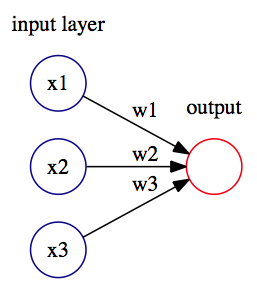
The perceptron was very promising, but it was soon discovered that is has serious limitations as it only works for linearly-separable classes. In 1969, Marvin Minsky and Seymour Papert demonstrated that it could not learn even a simple logical function such as XOR. This led to a significant decline in the interest in perceptron's.

However, other neural networks can solve this problem. A classic multilayer perceptron has multiple interconnected perceptron's, such as units that are organized in different sequential layers (input layer, one or more hidden layers, and an output layer). Each unit of a layer is connected to all units of the next layer. First, the information is presented to the input layer, then we use it to compute the output (or activation), y_i, for each unit of the first hidden layer. We propagate forward, with the output as input for the next layers in the network (hence feedforward), and so on until we reach the output. The most common way to train neural networks is with a gradient descent in combination with backpropagation. We'll discuss this in detail in chapter 2, Neural Networks.

The following diagram depicts the neural network with one hidden layer:

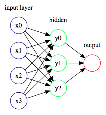
Think of the hidden layers as an abstract representation of the input data. This is the way the neural network understands the features of the data with its own internal logic. However, neural networks are non-interpretable models. This means that if we observed the y_i activations of the hidden layer, we wouldn't be able to understand them. For us, they are just a vector of numerical values. To bridge the gap between the network's representation and the actual data we're interested in, we need the output layer. You can think of this as a translator; we use it to understand the network's logic, and at the same time, we can convert it to the actual target values that we are interested in.

The Universal approximation theorem tells us that a feedforward network with one hidden layer can represent any function. It's good to know that there are no theoretical limits on networks with one hidden layer, but in practice we can achieve limited success with such architectures. In Chapter 3, Deep Learning Fundamentals, we'll discuss how to achieve better performance with deep neural networks, and their advantages over the shallow ones. For now, let's apply our knowledge by solving a simple classification task with a neural network.

In this section, we'll introduce PyTorch, version 1.0. PyTorch is an open source python deep learning framework, developed primarily by Facebook that has been gaining momentum recently. It provides the Graphics Processing Unit (GPU), an accelerated multidimensional array (or tensor) operation, and computational graphs, which we can be used to build neural networks. Throughout this book, we'll use PyTorch, TensorFlow, and Keras, and we'll talk in detail about these libraries and compare them in Chapter 3, Deep Learning Fundamentals.

The steps are as follows:

1. Let's create a simple neural network that will classify the Iris flower dataset. The following is the code block for creating a simple neural network:

import pandas as pd

dataset = pd.read_csv('https://archive.ics.uci.edu/ml/machine-learning-databases/iris/iris.data',
                      names=['sepal_length', 'sepal_width', 'petal_length', 'petal_width', 'species'])

dataset['species'] = pd.Categorical(dataset['species']).codes

dataset = dataset.sample(frac=1, random_state=1234)

train_input = dataset.values[:120, :4]
train_target = dataset.values[:120, 4]

test_input = dataset.values[120:, :4]
test_target = dataset.values[120:, 4]

2. The preceding code is boilerplate code that downloads the Iris dataset CSV file and then loads it into the pandas DataFrame. We then shuffle the DataFrame rows and split the code into numpy arrays, train_input/train_target (flower properties/flower class), for the training data and test_input/test_target for the test data.

3. We'll use 120 samples for training and 30 for testing. If you are not familiar with pandas, think of this as an advanced version of NumPy. Let's define our first neural network:

import torch

torch.manual_seed(1234)

hidden_units = 5

net = torch.nn.Sequential(
 torch.nn.Linear(4, hidden_units),
 torch.nn.ReLU(),
 torch.nn.Linear(hidden_units, 3)
)

4. We'll use a feedforward network with one hidden layer with five units, a ReLU activation function (this is just another type of activation, defined simply as f(x) = max(0, x)), and an output layer with three units. The output layer has three units, whereas each unit corresponds to one of the three classes of Iris flower. We'll use one-hot encoding for the target data. This means that each class of the flower will be represented as an array (Iris Setosa = [1, 0, 0], Iris Versicolour = [0, 1, 0], and Iris Virginica = [0, 0, 1]), and one element of the array will be the target for one unit of the output layer. When the network classifies a new sample, we'll determine the class by taking the unit with the highest activation value.
5. torch.manual_seed(1234) enables us to use the same random data every time for the reproducibility of results.
6. Choose the optimizer and loss function:

# choose optimizer and loss function
criterion = torch.nn.CrossEntropyLoss()
optimizer = torch.optim.SGD(net.parameters(), lr=0.1, momentum=0.9)

7. With the criterion variable, we define the loss function that we'll use, in this case, this is cross-entropy loss. The loss function will measure how different the output of the network is compared to the target data.

8. We then define the stochastic gradient descent (SGD) optimizer with a learning rate of 0.1 and a momentum of 0.9. The SGD is a variation of the gradient descent algorithm. We'll discuss loss functions and SGD in detail in Chapter 2, Neural Networks. Now, let's train the network:

# train
epochs = 50

for epoch in range(epochs):
 inputs = torch.autograd.Variable(torch.Tensor(train_input).float())
 targets = torch.autograd.Variable(torch.Tensor(train_target).long())

 optimizer.zero_grad()
 out = net(inputs)
 loss = criterion(out, targets)
 loss.backward()
 optimizer.step()

 if epoch == 0 or (epoch + 1) % 10 == 0:
 print('Epoch %d Loss: %.4f' % (epoch + 1, loss.item()))

9. We'll run the training for 50 epochs, which means that we'll iterate 50 times over the training dataset:
   1. Create the torch variable that are input and target from the numpy array train_input and train_target.
   2. Zero the gradients of the optimizer to prevent accumulation from the previous iterations. We feed the training data to the neural network net (input) and we compute the loss function criterion (out, targets) between the network output and the target data.
   3. Propagate the loss value back through the network. We do this so that we can calculate how each network weight affects the loss function.
   4. The optimizer updates the weights of the network in a way that will reduce the future loss function values.

When we run the training, the output is as follows:

Epoch 1 Loss: 1.2181
Epoch 10 Loss: 0.6745
Epoch 20 Loss: 0.2447
Epoch 30 Loss: 0.1397
Epoch 40 Loss: 0.1001
Epoch 50 Loss: 0.0855

In the following graph, you can see how the loss function decreases with each epoch. This shows how the network gradually learns the training data:

10. Let's see what the final accuracy of our model is:

import numpy as np

inputs = torch.autograd.Variable(torch.Tensor(test_input).float())
targets = torch.autograd.Variable(torch.Tensor(test_target).long())

optimizer.zero_grad()
out = net(inputs)
_, predicted = torch.max(out.data, 1)

error_count = test_target.size - np.count_nonzero((targets == predicted).numpy())
print('Errors: %d; Accuracy: %d%%' % (error_count, 100 * torch.sum(targets == predicted) / test_target.size))

We do this by feeding the test set to the network and computing the error manually. The output is as follows:

Errors: 0; Accuracy: 100%

We were able to classify all 30 test samples correctly.

We must also keep in mind trying different hyperparameters of the network and see how the accuracy and loss functions work. You could try changing the number of units in the hidden layer, the number of epochs we train in the network, as well as the learning rate.