Book Image

Learning OpenCV 4 Computer Vision with Python 3 - Third Edition

By : Joseph Howse, Joe Minichino
Book Image

Learning OpenCV 4 Computer Vision with Python 3 - Third Edition

By: Joseph Howse, Joe Minichino

Overview of this book

Computer vision is a rapidly evolving science, encompassing diverse applications and techniques. This book will not only help those who are getting started with computer vision but also experts in the domain. You’ll be able to put theory into practice by building apps with OpenCV 4 and Python 3. You’ll start by understanding OpenCV 4 and how to set it up with Python 3 on various platforms. Next, you’ll learn how to perform basic operations such as reading, writing, manipulating, and displaying still images, videos, and camera feeds. From taking you through image processing, video analysis, and depth estimation and segmentation, to helping you gain practice by building a GUI app, this book ensures you’ll have opportunities for hands-on activities. Next, you’ll tackle two popular challenges: face detection and face recognition. You’ll also learn about object classification and machine learning concepts, which will enable you to create and use object detectors and classifiers, and even track objects in movies or video camera feed. Later, you’ll develop your skills in 3D tracking and augmented reality. Finally, you’ll cover ANNs and DNNs, learning how to develop apps for recognizing handwritten digits and classifying a person's gender and age. By the end of this book, you’ll have the skills you need to execute real-world computer vision projects.
Table of Contents (13 chapters)

Basic I/O scripts

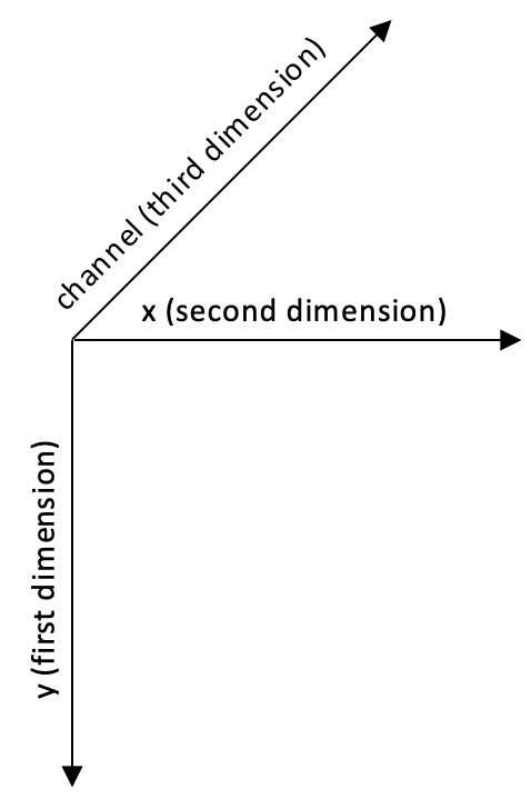
Most CV applications need to get images as input. Most also produce images as output. An interactive CV application might require a camera as an input source and a window as an output destination. However, other possible sources and destinations include image files, video files, and raw bytes. For example, raw bytes might be transmitted via a network connection, or they might be generated by an algorithm if we incorporate procedural graphics into our application. Let's look at each of these possibilities.

Reading/writing an image file

OpenCV provides the imread function to load an image from a file and the imwrite function to write an image to a file. These functions support various file formats for still images (not videos). The supported formats vary—as formats can be added or removed in a custom build of OpenCV—but normally BMP, PNG, JPEG, and TIFF are among the supported formats.

Let's explore the anatomy of the representation of an image in OpenCV and NumPy. An image is a multidimensional array; it has columns and rows of pixels, and each pixel has a value. For different kinds of image data, the pixel value may be formatted in different ways. For example, we can create a 3x3 square black image from scratch by simply creating a 2D NumPy array:

img = numpy.zeros((3, 3), dtype=numpy.uint8)

If we print this image to a console, we obtain the following result:

array([[0, 0, 0],
[0, 0, 0],
[0, 0, 0]], dtype=uint8)

Here, each pixel is represented by a single 8-bit integer, which means that the values for each pixel are in the 0-255 range, where 0 is black, 255 is white, and the in-between values are shades of gray. This is a grayscale image.

Let's now convert this image into blue-green-red (BGR) format using the cv2.cvtColor function:

img = cv2.cvtColor(img, cv2.COLOR_GRAY2BGR)

Let's observe how the image has changed:

array([[[0, 0, 0],
[0, 0, 0],
[0, 0, 0]],

[[0, 0, 0],
[0, 0, 0],
[0, 0, 0]],

[[0, 0, 0],
[0, 0, 0],
[0, 0, 0]]], dtype=uint8)

As you can see, each pixel is now represented by a three-element array, with each integer representing one of the three color channels: B, G, and R, respectively. Other common color models, such as HSV, will be represented in the same way, albeit with different value ranges. For example, the hue value of the HSV color model has a range of 0-180.

For more information about color models, refer to Chapter 3, Processing Images with OpenCV, specifically the Converting between different color models section.

You can check the structure of an image by inspecting the shape property, which returns rows, columns, and the number of channels (if there is more than one).

Consider this example:

img = numpy.zeros((5, 3), dtype=numpy.uint8)
print(img.shape)

The preceding code will print (5, 3); in other words, we have a grayscale image with 5 rows and 3 columns. If you then converted the image into BGR, the shape would be (5, 3, 3), which indicates the presence of three channels per pixel.

Images can be loaded from one file format and saved to another. For example, let's convert an image from PNG into JPEG:

import cv2

image = cv2.imread('MyPic.png')
cv2.imwrite('MyPic.jpg', image)
OpenCV's Python module is called cv2 even though we are using OpenCV 4.x and not OpenCV 2.x. Historically, OpenCV had two Python modules: cv2 and cv. The latter wrapped a legacy version of OpenCV implemented in C. Nowadays, OpenCV has only the cv2 Python module, which wraps the current version of OpenCV implemented in C++.

By default, imread returns an image in the BGR color format even if the file uses a grayscale format. BGR represents the same color model as red-green-blue (RGB), but the byte order is reversed.

Optionally, we may specify the mode of imread. The supported options include the following:

  • cv2.IMREAD_COLOR: This is the default option, providing a 3-channel BGR image with an 8-bit value (0-255) for each channel.
  • cv2.IMREAD_GRAYSCALE: This provides an 8-bit grayscale image.
  • cv2.IMREAD_ANYCOLOR: This provides either an 8-bit-per-channel BGR image or an 8-bit grayscale image, depending on the metadata in the file.
  • cv2.IMREAD_UNCHANGED: This reads all of the image data, including the alpha or transparency channel (if there is one) as a fourth channel.
  • cv2.IMREAD_ANYDEPTH: This loads an image in grayscale at its original bit depth. For example, it provides a 16-bit-per-channel grayscale image if the file represents an image in this format.
  • cv2.IMREAD_ANYDEPTH | cv2.IMREAD_COLOR: This combination loads an image in BGR color at its original bit depth.
  • cv2.IMREAD_REDUCED_GRAYSCALE_2: This loads an image in grayscale at half its original resolution. For example, if the file contains a 640 x 480 image, it is loaded as a 320 x 240 image.
  • cv2.IMREAD_REDUCED_COLOR_2: This loads an image in 8-bit-per-channel BGR color at half its original resolution.
  • cv2.IMREAD_REDUCED_GRAYSCALE_4: This loads an image in grayscale at one-quarter of its original resolution.
  • cv2.IMREAD_REDUCED_COLOR_4: This loads an image in 8-bit-per-channel color at one-quarter of its original resolution.
  • cv2.IMREAD_REDUCED_GRAYSCALE_8: This loads an image in grayscale at one-eighth of its original resolution.
  • cv2.IMREAD_REDUCED_COLOR_8: This loads an image in 8-bit-per-channel color at one-eighth of its original resolution.

As an example, let's load a PNG file as a grayscale image (losing any color information in the process), and then save it as a grayscale PNG image:

import cv2

grayImage = cv2.imread('MyPic.png', cv2.IMREAD_GRAYSCALE)
cv2.imwrite('MyPicGray.png', grayImage)

The path of an image, unless absolute, is relative to the working directory (the path from which the Python script is run), so, in the preceding example, MyPic.png would have to be in the working directory or the image would not be found. If you prefer to avoid assumptions about the working directory, you can use absolute paths, such as C:\Users\Joe\Pictures\MyPic.png on Windows, /Users/Joe/Pictures/MyPic.png on Mac, or /home/joe/pictures/MyPic.png on Linux.

The imwrite() function requires an image to be in the BGR or grayscale format with a certain number of bits per channel that the output format can support. For example, the BMP file format requires 8 bits per channel, while PNG allows either 8 or 16 bits per channel.

Converting between an image and raw bytes

Conceptually, a byte is an integer ranging from 0 to 255. Throughout real-time graphic applications today, a pixel is typically represented by one byte per channel, though other representations are also possible.

An OpenCV image is a 2D or 3D array of the numpy.array type. An 8-bit grayscale image is a 2D array containing byte values. A 24-bit BGR image is a 3D array, which also contains byte values. We may access these values by using an expression such as image[0, 0] or image[0, 0, 0]. The first index is the pixel's y coordinate or row, 0 being the top. The second index is the pixel's x coordinate or column, 0 being the leftmost. The third index (if applicable) represents a color channel. The array's three dimensions can be visualized in the following Cartesian coordinate system:

For example, in an 8-bit grayscale image with a white pixel in the upper-left corner, image[0, 0] is 255. For a 24-bit (8-bit-per-channel) BGR image with a blue pixel in the upper-left corner, image[0, 0] is [255, 0, 0].

Provided that an image has 8 bits per channel, we can cast it to a standard Python bytearray object, which is one-dimensional:

byteArray = bytearray(image)

Conversely, provided that bytearray contains bytes in an appropriate order, we can cast and then reshape it to get a numpy.array type that is an image:

grayImage = numpy.array(grayByteArray).reshape(height, width)
bgrImage = numpy.array(bgrByteArray).reshape(height, width, 3)

As a more complete example, let's convert bytearray that contains random bytes into a grayscale image and a BGR image:

import cv2
import numpy
import os

# Make an array of 120,000 random bytes.
randomByteArray = bytearray(os.urandom(120000))
flatNumpyArray = numpy.array(randomByteArray)

# Convert the array to make a 400x300 grayscale image.
grayImage = flatNumpyArray.reshape(300, 400)
cv2.imwrite('RandomGray.png', grayImage)

# Convert the array to make a 400x100 color image.
bgrImage = flatNumpyArray.reshape(100, 400, 3)
cv2.imwrite('RandomColor.png', bgrImage)
Here, we use Python's standard os.urandom function to generate random raw bytes, which we then convert into a NumPy array. Note that it is also possible to generate a random NumPy array directly (and more efficiently) using a statement such as numpy.random.randint(0, 256, 120000).reshape(300, 400). The only reason we use os.urandom is to help to demonstrate conversion from raw bytes.

After running this script, we should have a pair of randomly generated images, RandomGray.png and RandomColor.png, in the script's directory.

Here is an example of RandomGray.png (though yours will almost certainly differ since it is random):

Similarly, here is an example of RandomColor.png:

Now that we have a better understanding of how an image is formed from data, we can start performing basic operations on it.

Accessing image data with numpy.array

We already know that the easiest (and most common) way to load an image in OpenCV is to use the imread function. We also know that this will return an image, which is really an array (either a 2D or 3D one, depending on the parameters you passed to imread).

The numpy.array class is greatly optimized for array operations, and it allows certain kinds of bulk manipulations that are not available in a plain Python list. These kinds of numpy.array type-specific operations come in handy for image manipulations in OpenCV. However, let's explore image manipulations step by step, starting with a basic example. Say you want to manipulate a pixel at coordinates (0, 0) in a BGR image and turn it into a white pixel:

import cv2

img = cv2.imread('MyPic.png')
img[0, 0] = [255, 255, 255]

If you then save the modified image to file and view it, you will see a white dot in the top-left corner of the image. Naturally, this modification is not very useful, but it begins to show the possibilities. Now, let's leverage the capabilities of numpy.array to perform transformations on an array much faster than we could do with a plain Python list.

Let's say that you want to change the blue value of a particular pixel, say, the pixel at coordinates, (150, 120). The numpy.array type provides a handy method, item, which takes three parameters: the x (or left) position, the y (or top) position, and the index within the array at the (x, y) position (remember that in a BGR image, the data at a certain position is a three-element array containing the B, G, and R values in this order) and returns the value at the index position. Another method, itemset, sets the value of a particular channel of a particular pixel to a specified value. itemset takes two arguments: a three-element tuple (x, y, and index) and the new value.

In the following example, we change the value of the blue channel at (150, 120) from its current value to an arbitrary 255:

import cv2

img = cv2.imread('MyPic.png')
img.itemset((150, 120, 0), 255) # Sets the value of a pixel's blue channel
print(img.item(150, 120, 0)) # Prints the value of a pixel's blue channel

For modifying a single element in an array, the itemset method is somewhat faster than the indexing syntax that we saw in the first example in this section.

Again, modifying an element of an array does not do much in itself, but it does open a world of possibilities. However, for performance reasons, this is only suitable for small regions of interest. When you need to manipulate an entire image or a large region of interest, it is advisable that you utilize either OpenCV's functions or NumPy's array slicing. The latter allows you to specify a range of indices. Let's consider an example of using array slicing to manipulate color channels. Setting all G (green) values of an image to 0 is as simple as the following code:

import cv2

img = cv2.imread('MyPic.png')
img[:, :, 1] = 0

This piece of code performs a fairly significant operation and is easy to understand. The relevant line is the last one, which basically instructs the program to take all pixels from all rows and columns and set the green value (at index one of the three-element BGR array) to 0. If you display this image, you will notice a complete absence of green.

There are several interesting things we can do by accessing raw pixels with NumPy's array slicing; one of them is defining regions of interests (ROI). Once the region is defined, we can perform a number of operations. For example, we can bind this region to a variable, define a second region, and assign the value of the first region to the second (hence, copying a portion of the image over to another position in the image):

import cv2

img = cv2.imread('MyPic.png')
my_roi = img[0:100, 0:100]
img[300:400, 300:400] = my_roi

It is important to make sure that the two regions correspond in terms of size. If not, NumPy will (rightly) complain that the two shapes are mismatched.

Finally, we can access the properties of numpy.array, as shown in the following code:

import cv2

img = cv2.imread('MyPic.png')
print(img.shape)
print(img.size)
print(img.dtype)

These three properties are defined as follows:

  • shape: This is a tuple describing the shape of the array. For an image, it contains (in order) the height, width, and—if the image is in colorthe number of channels. The length of the shape tuple is a useful way to determine whether an image is grayscale or color. For a grayscale image, we have len(shape) == 2, and for a color image, len(shape) == 3.
  • size: This is the number of elements in the array. In the case of a grayscale image, this is the same as the number of pixels. In the case of a BGR image, it is three times the number of pixels because each pixel is represented by three elements (B, G, and R).
  • dtype: This is the datatype of the array's elements. For an 8-bit-per-channel image, the datatype is numpy.uint8.

All in all, it is strongly advised that you familiarize yourself with NumPy in general, and numpy.array in particular, when working with OpenCV. This class is the foundation of any image processing done with OpenCV in Python.

Reading/writing a video file

OpenCV provides the VideoCapture and VideoWriter classes, which support various video file formats. The supported formats vary depending on the operating system and the build configuration of OpenCV, but normally it is safe to assume that the AVI format is supported. Via its read method, a VideoCapture object may be polled for new frames until it reaches the end of its video file. Each frame is an image in a BGR format.

Conversely, an image may be passed to the write method of the VideoWriter class, which appends the image to a file in VideoWriter. Let's look at an example that reads frames from one AVI file and writes them to another with a YUV encoding:

import cv2

videoCapture = cv2.VideoCapture('MyInputVid.avi')
fps = videoCapture.get(cv2.CAP_PROP_FPS)
size = (int(videoCapture.get(cv2.CAP_PROP_FRAME_WIDTH)),
int(videoCapture.get(cv2.CAP_PROP_FRAME_HEIGHT)))
videoWriter = cv2.VideoWriter(
'MyOutputVid.avi', cv2.VideoWriter_fourcc('I','4','2','0'),
fps, size)

success, frame = videoCapture.read()
while success: # Loop until there are no more frames.
videoWriter.write(frame)
success, frame = videoCapture.read()

The arguments to the constructor of the VideoWriter class deserve special attention. A video's filename must be specified. Any preexisting file with this name is overwritten. A video codec must also be specified. The available codecs may vary from system to system. The supported options may include the following:

  • 0: This option is an uncompressed raw video file. The file extension should be .avi.
  • cv2.VideoWriter_fourcc('I','4','2','0'): This option is an uncompressed YUV encoding, 4:2:0 chroma subsampled. This encoding is widely compatible but produces large files. The file extension should be .avi.
  • cv2.VideoWriter_fourcc('P','I','M','1'): This option is MPEG-1. The file extension should be .avi.
  • cv2.VideoWriter_fourcc('X','V','I','D'): This option is a relatively old MPEG-4 encoding. It is a good option if you want to limit the size of the resulting video. The file extension should be .avi.
  • cv2.VideoWriter_fourcc('M','P','4','V'): This option is another relatively old MPEG-4 encoding. It is a good option if you want to limit the size of the resulting video. The file extension should be .mp4.
  • cv2.VideoWriter_fourcc('X','2','6','4'): This option is a relatively new MPEG-4 encoding. It may be the best option if you want to limit the size of the resulting video. The file extension should be .mp4.
  • cv2.VideoWriter_fourcc('T','H','E','O'): This option is Ogg Vorbis. The file extension should be .ogv.
  • cv2.VideoWriter_fourcc('F','L','V','1'): This option is a Flash video. The file extension should be .flv.

A frame rate and frame size must be specified too. Since we are copying from another video, these properties can be read from the get method of the VideoCapture class.

Capturing camera frames

A stream of camera frames is represented by a VideoCapture object too. However, for a camera, we construct a VideoCapture object by passing the camera's device index instead of a video's filename. Let's consider the following example, which captures 10 seconds of video from a camera and writes it to an AVI file. The code is similar to the previous section's sample (which was captured from a video file instead of a camera) but changes are marked in bold:

import cv2

cameraCapture = cv2.VideoCapture(0)
fps = 30 # An assumption
size = (int(cameraCapture.get(cv2.CAP_PROP_FRAME_WIDTH)),
int(cameraCapture.get(cv2.CAP_PROP_FRAME_HEIGHT)))
videoWriter = cv2.VideoWriter(
'MyOutputVid.avi', cv2.VideoWriter_fourcc('I','4','2','0'),
fps, size)

success, frame = cameraCapture.read()
numFramesRemaining = 10 * fps - 1 # 10 seconds of frames
while success and numFramesRemaining > 0:
videoWriter.write(frame)
success, frame = cameraCapture.read()
numFramesRemaining -= 1

For some cameras on certain systems, cameraCapture.get(cv2.CAP_PROP_FRAME_WIDTH) and cameraCapture.get(cv2.CAP_PROP_FRAME_HEIGHT) may return inaccurate results. To be more certain of the actual image dimensions, you can first capture a frame and then get its height and width with code such as h, w = frame.shape[:2]. Occasionally, you might even encounter a camera that yields a few bad frames with unstable dimensions before it starts yielding good frames with stable dimensions. If you are concerned about guarding against this kind of quirk, you may want to read and ignore a few frames at the start of a capture session.

Unfortunately, in most cases, the get method of VideoCapture does not return an accurate value for the camera's frame rate; it typically returns 0. The official documentation at http://docs.opencv.org/modules/highgui/doc/reading_and_writing_images_and_video.html warns of the following:

"Value 0 is returned when querying a property that is not supported by the backend used by the VideoCapture instance.

Note
Reading / writing properties involves many layers. Some unexpected result might happens [sic] along this chain.
VideoCapture -> API Backend -> Operating System -> Device Driver -> Device Hardware
The returned value might be different from what really is used by the device or it could be encoded using device-dependent rules (for example, steps or percentage). Effective behavior depends from [sic] device driver and the API backend."

To create an appropriate VideoWriter class for the camera, we have to either make an assumption about the frame rate (as we did in the preceding code) or measure it using a timer. The latter approach is better and we will cover it later in this chapter.

The number of cameras and their order is, of course, system-dependent. Unfortunately, OpenCV does not provide any means of querying the number of cameras or their properties. If an invalid index is used to construct a VideoCapture class, the VideoCapture class will not yield any frames; its read method will return (False, None). To avoid trying to retrieve frames from a VideoCapture object that was not opened correctly, you may want to first call the VideoCapture.isOpened method, which returns a Boolean.

The read method is inappropriate when we need to synchronize either a set of cameras or a multihead camera such as a stereo camera. Then, we use the grab and retrieve methods instead. For a set of two cameras, we can use code similar to the following:

success0 = cameraCapture0.grab()
success1 = cameraCapture1.grab()
if success0 and success1:
frame0 = cameraCapture0.retrieve()
frame1 = cameraCapture1.retrieve()

Displaying an image in a window

One of the most basic operations in OpenCV is displaying an image in a window. This can be done with the imshow function. If you come from any other GUI framework background, you might think it sufficient to call imshow to display an image. However, in OpenCV, the window is drawn (or re-drawn) only when you call another function, waitKey. The latter function pumps the window's event queue (allowing various events such as drawing to be handled), and it returns the keycode of any key that the user may have typed within a specified timeout. To some extent, this rudimentary design simplifies the task of developing demos that use video or webcam input; at least the developer has manual control over the capture and display of new frames.

Here is a very simple sample script to read an image from a file and display it:

import cv2
import numpy as np

img = cv2.imread('my-image.png')
cv2.imshow('my image', img)
cv2.waitKey()
cv2.destroyAllWindows()

The imshow function takes two parameters: the name of the window in which we want to display the image and the image itself. We will talk about waitKey in more detail in the next section, Displaying camera frames in a window.

The aptly named destroyAllWindows function disposes of all of the windows created by OpenCV.

Displaying camera frames in a window

OpenCV allows named windows to be created, redrawn, and destroyed using the namedWindow, imshow, and destroyWindow functions. Also, any window may capture keyboard input via the waitKey function and mouse input via the setMouseCallback function. Let's look at an example where we show the frames captured from a live camera:

import cv2

clicked = False
def onMouse(event, x, y, flags, param):
global clicked
if event == cv2.EVENT_LBUTTONUP:
clicked = True

cameraCapture = cv2.VideoCapture(0)
cv2.namedWindow('MyWindow')
cv2.setMouseCallback('MyWindow', onMouse)

print('Showing camera feed. Click window or press any key to stop.')
success, frame = cameraCapture.read()
while success and cv2.waitKey(1) == -1 and not clicked:
cv2.imshow('MyWindow', frame)
success, frame = cameraCapture.read()

cv2.destroyWindow('MyWindow')
cameraCapture.release()

The argument for waitKey is a number of milliseconds to wait for keyboard input. By default, it is 0, which is a special value meaning infinity. The return value is either -1 (meaning that no key has been pressed) or an ASCII keycode, such as 27 for Esc. For a list of ASCII keycodes, refer to http://www.asciitable.com/. Also, note that Python provides a standard function, ord, which can convert a character into its ASCII keycode. For example, ord('a') returns 97.

Again, note that OpenCV's window functions and waitKey are interdependent. OpenCV windows are only updated when waitKey is called. Conversely, waitKey only captures input when an OpenCV window has focus.

The mouse callback passed to setMouseCallback should take five arguments, as seen in our code sample. The callback's param argument is set as an optional third argument to setMouseCallback. By default, it is 0. The callback's event argument is one of the following actions:

  • cv2.EVENT_MOUSEMOVE: This event refers to mouse movement.
  • cv2.EVENT_LBUTTONDOWN: This event refers to the left button going down when it is pressed.
  • cv2.EVENT_RBUTTONDOWN: This event refers to the right button going down when it is pressed.
  • cv2.EVENT_MBUTTONDOWN: This event refers to the middle button going down when it is pressed.
  • cv2.EVENT_LBUTTONUP: This event refers to the left button coming back up when it is released.
  • cv2.EVENT_RBUTTONUP: This event refers to the right button coming back up when it is released.
  • cv2.EVENT_MBUTTONUP: This event refers to the middle button coming back up when it is released.
  • cv2.EVENT_LBUTTONDBLCLK: This event refers to the left button being double-clicked.
  • cv2.EVENT_RBUTTONDBLCLK: This event refers to the right button being double-clicked.
  • cv2.EVENT_MBUTTONDBLCLK: This event refers to the middle button being double-clicked.

The mouse callback's flags argument may be some bitwise combination of the following events:

  • cv2.EVENT_FLAG_LBUTTON: This event refers to the left button being pressed.
  • cv2.EVENT_FLAG_RBUTTON: This event refers to the right button being pressed.
  • cv2.EVENT_FLAG_MBUTTON: This event refers to the middle button being pressed.
  • cv2.EVENT_FLAG_CTRLKEY: This event refers to the Ctrl key being pressed.
  • cv2.EVENT_FLAG_SHIFTKEY: This event refers to the Shift key being pressed.
  • cv2.EVENT_FLAG_ALTKEY: This event refers to the Alt key being pressed.

Unfortunately, OpenCV does not provide any means of manually handling window events. For example, we cannot stop our application when a window's close button is clicked. Due to OpenCV's limited event handling and GUI capabilities, many developers prefer to integrate it with other application frameworks. Later in this chapter, in the Cameo – an object-oriented design section, we will design an abstraction layer to help to integrate OpenCV with any application framework.