Long exposure (or light art) refers to the process of creating a photo that captures the effect of passing time. Some popular application examples of long exposure photographs are silky-smooth water and a single band of continuous-motion illumination of the highways with car headlights. In this recipe, we will simulate the long exposures by averaging the image frames from a video.

We will extract image frames from a video and then average the frames to simulate light art. Let's start by importing the required libraries:

from glob import glob
import cv2
import numpy as np
import matplotlib.pylab as plt

The following steps need to be performed:

1. Implement an extract_frames() function to extract the first 200 frames (at most) from a video passed as input to the function:

def extract_frames(vid_file):
 vidcap = cv2.VideoCapture(vid_file)
 success,image = vidcap.read()
 i = 1
 success = True
 while success and i <= 200:
  cv2.imwrite('images/exposure/vid_{}.jpg'.format(i), image)
  success,image = vidcap.read()
  i += 1

2. Call the function to save all of the frames (as .jpg) extracted from the video of the waterfall in Godafost (Iceland) to the exposure folder:

extract_frames('images/godafost.mp4') #cloud.mp4

3. Read all the .jpg files from the exposure folder; read them one by one (as float); split each image into B, G, and R channels; compute a running sum of the color channels; and finally, compute average values for the color channels:

imfiles = glob('images/exposure/*.jpg')
nfiles = len(imfiles)
R1, G1, B1 = 0, 0, 0
for i in range(nfiles):
 image = cv2.imread(imfiles[i]).astype(float)
 (B, G, R) = cv2.split(image)
 R1 += R
 B1 += B
 G1 += G
R1, G1, B1 = R1 / nfiles, G1 / nfiles, B1 / nfiles

4. Merge the average values of the color channels obtained and save the final output image:

final = cv2.merge([B1, G1, R1])
cv2.imwrite('images/godafost.png', final)

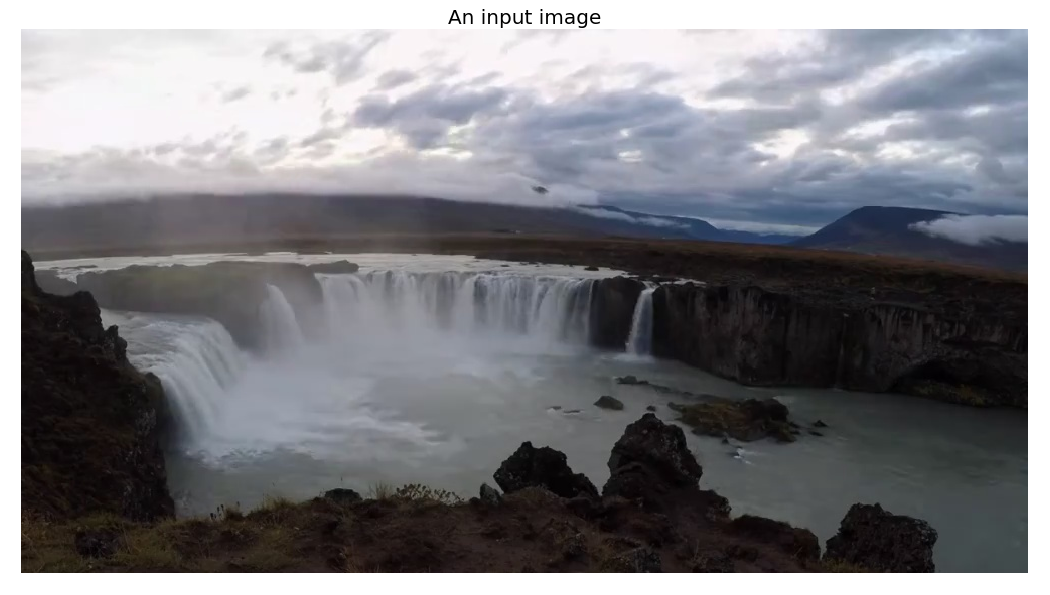
The following photo shows one of the extracted input frames:

If you run the preceding code block, you will obtain a long exposure-like image like the one shown here:

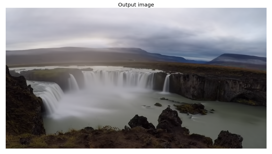
Notice the continuous effects in the clouds and the waterfall.

The VideoCapture() function from OpenCV-Python was used to create a VideoCapture object with the video file as input. Then, the read() method of that object was used to capture frames from the video.

The imread() and imwrite() functions from OpenCV-Python were used to read/write images from/to disk.

The cv2.split() function was used to split an RGB image into individual color channels, while the cv2.merge() function was used to combine them back into an RGB image.

Focus stacking (also known as extended depth of fields) is a technique (in image processing/computational photography) that takes multiple images (of the same subject but captured at different focus distances) as input and then creates an output image with a higher DOF than any of the individual source images by combining the input images. We can simulate focus stacking in Python. The following is an example of focus stacking grayscale image frames extracted from a video using the mahotas library.

Perform the following steps to implement focus stacking with the mahotas library functions:

1. Create the image stack first by extracting grayscale image frames from a highway traffic video at night:

import mahotas as mh
def create_image_stack(vid_file, n = 200): 
 vidcap = cv2.VideoCapture(vid_file)
 success,image = vidcap.read()
 i = 0
 success = True
 h, w = image.shape[:2]
 imstack = np.zeros((n, h, w))
 while success and i < n:
   imstack[i,...] = cv2.cvtColor(image, cv2.COLOR_BGR2GRAY)
   success,image = vidcap.read()
   i += 1
 return imstack

image = create_image_stack('images/highway.mp4') #cloud.mp4
stack,h,w = image.shape

2. Use the sobel() function from mahotas as the pixel-level measure of infocusness:

focus = np.array([mh.sobel(t, just_filter=True) for t in image])

3. At each pixel location, select the best slice (with maximum infocusness) and create the final image:

best = np.argmax(focus, 0)
image = image.reshape((stack,-1)) # image is now (stack, nr_pixels)
image = image.transpose() # image is now (nr_pixels, stack)
final = image[np.arange(len(image)), best.ravel()] # Select the right pixel at each location
final = final.reshape((h,w)) # reshape to get final result

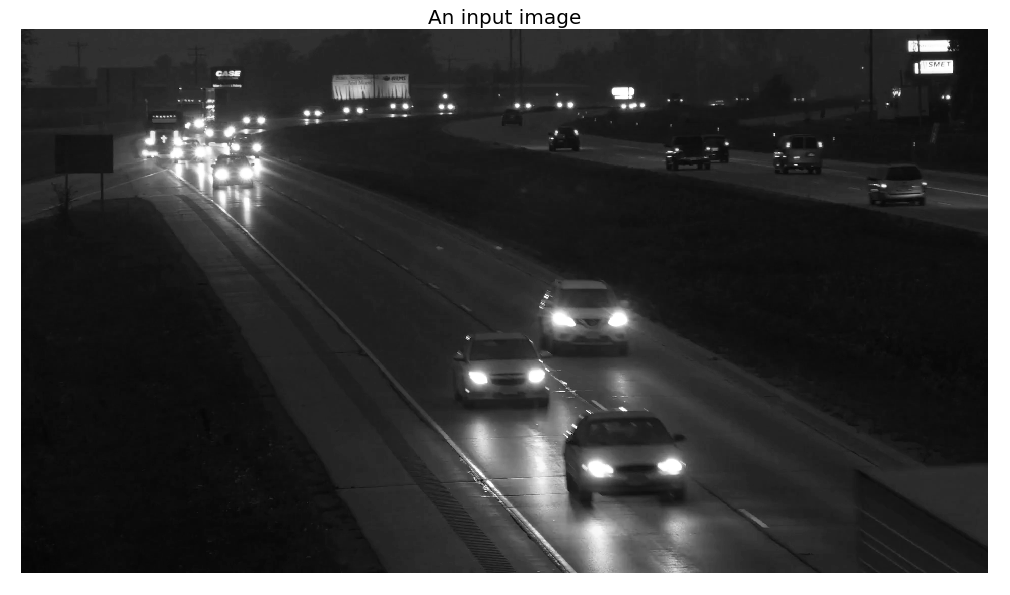
The following photo is an input image used in the image stack:

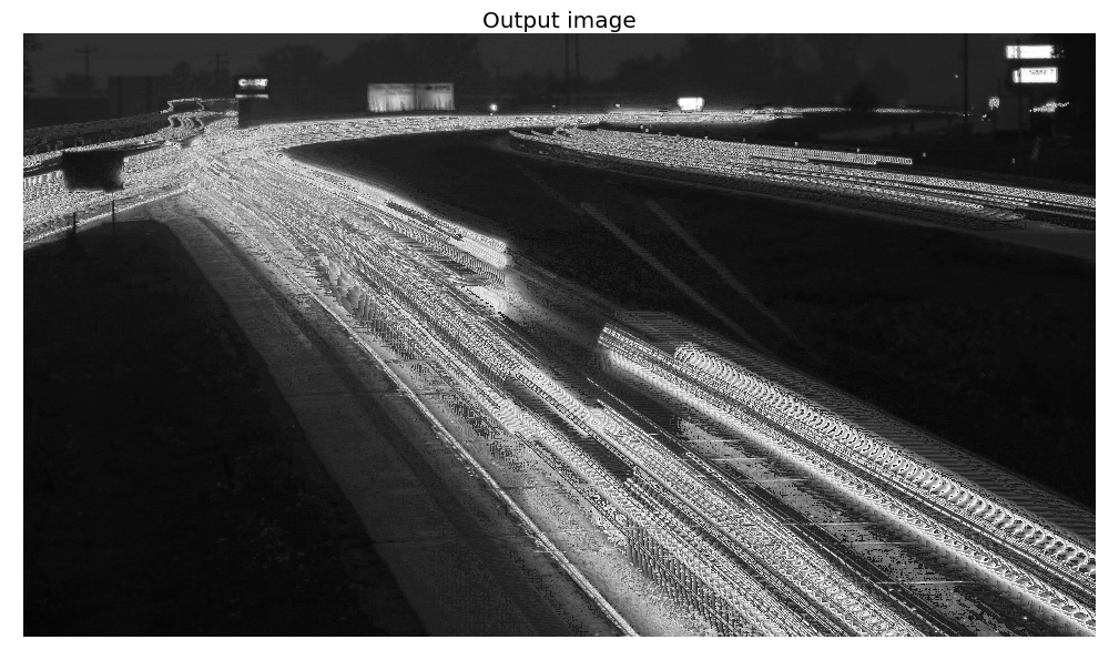
The following screenshot is the final output image produced by the algorithm implementation:

For more details, refer to the following links:

• https://mahotas.readthedocs.io/en/latest/edf.html
• https://docs.opencv.org/3.0-beta/doc/py_tutorials/py_gui/py_video_display/py_video_display.html
• https://www.youtube.com/watch?v=5CTSc9GX3X8