Initially known as IPython, this project was initiated in 2001 as a free project by Fernando Perez. By his work, the author intended to address a lack in the Python stack and provide to the public a user programming interface for data investigations that could easily incorporate the scientific approach (mainly meaning experimenting and interactively discovering) in the process of data discovery and software development.

A scientific approach implies fast experimentation of different hypotheses in a reproducible fashion (as does data exploration and analysis in data science), and when using this interface, you will be able more naturally to implement an explorative, iterative, trial and error research strategy during your code writing.

Recently (during Spring 2015), a large part of the IPython project was moved to a new one called Jupyter. This new project extends the potential usability of the original IPython interface to a wide range of programming languages, such as these:

• R (https://github.com/IRkernel/IRkernel)
• Julia (http://github.com/JuliaLang/IJulia.jl)
• Scala (https://github.com/mattpap/IScala)

For a more complete list of available kernels for Jupyter, please visit https://github.com/ipython/ipython/wiki/IPython-kernels-for-other-languages.

For instance, once having installed Jupyter and its IPython kernel, you can easily add another useful kernel, such as the R kernel, in order to access the R language through the same interface. All you have to do is have an R installation, run your R interface, and enter the following commands:

install.packages(c('pbdZMQ', 'devtools'))
devtools::install_github('IRkernel/repr')
devtools::install_github('IRkernel/IRdisplay')
devtools::install_github('IRkernel/IRkernel')
IRkernel::installspec()

The commands will install the devtools library on your R, then pull and install all the necessary libraries from GitHub (you need to be connected to the internet while running the other commands), and finally register the R kernel both in your R installation and on Jupyter. After that, every time you call the Jupyter Notebook, you will have the choice of running either a Python or an R kernel, allowing you to use the same format and approach for all your data science projects.

Thanks to the powerful idea of kernels, programs that run the user's code that's communicated by the frontend interface and provide feedback on the results of the executed code to the interface itself, you can use the same interface and interactive programming style no matter what language you are using for development.

In such a context, IPython is the zero kernel, the original starting one, still existing but not intended to be used anymore to refer to the entire project.

Therefore, Jupyter can simply be described as a tool for interactive tasks that are operable by a console or by a web-based notebook, which offers special commands that help developers to better understand and build the code that is being currently written.

Contrary to an IDE—which is built around the idea of writing a script, running it afterward, and finally evaluating its results—Jupyter lets you write your code in chunks, named cells, run each of them sequentially, and evaluate the results of each one separately, examining both textual and graphical outputs. Besides graphical integration, it provides you with further help, thanks to customizable commands, a rich history (in the JSON format), and computational parallelism for an enhanced performance when dealing with heavy numeric computations.

Such an approach is also particularly fruitful for tasks involving developing code based on data, since it automatically accomplishes the often neglected duty of documenting and illustrating how data analysis has been done, its premises and assumptions, and its intermediate and final results. If a part of your job is to also present your work and persuade an internal or external stakeholder in the project, Jupyter can really do the magic of storytelling for you with little additional effort.

You can easily combine code, comments, formulas, charts, interactive plots, and rich media such as images and videos, making each Jupyter Notebook a complete scientific sketchpad to find all your experimentations and their results together.

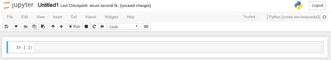
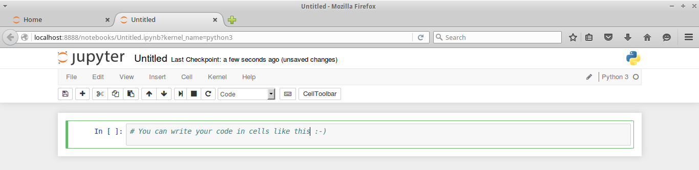
Jupyter works on your favorite browser (which could be Explorer, Firefox, or Chrome, for instance) and, when started, presents a cell waiting for code to be written in. Each block of code enclosed in a cell can be run, and its results are reported in the space just after the cell. Plots can be represented in the notebook (inline plot) or in a separate window. In our example, we decided to plot our chart inline.

Moreover, written notes can be written easily using the Markdown language, a very easy and fast-to-grasp markup language (http://daringfireball.net/projects/markdown/). Math formulas can be handled using MathJax (https://www.mathjax.org/) to render any LaTeX script inside HTML/markdown.

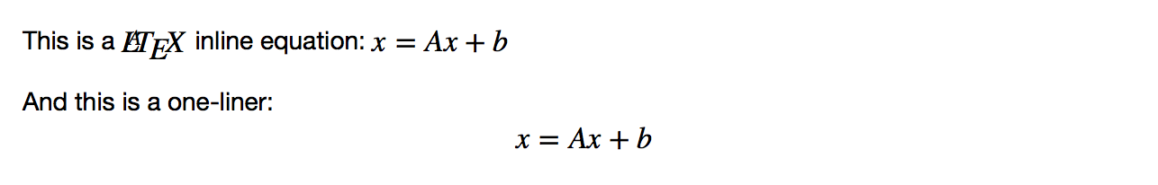
There are several ways to insert LaTeX code in a cell. The easiest way is to simply use the Markdown syntax, wrapping the equations with a single dollar sign, $, for an inline LaTeX formula, or with a double dollar sign, $$, for a one-line central equation. Remember that to have a correct output, the cell should be set as Markdown. Here's an example:

In Markdown:

This is a $LaTeX$ inline equation: $x = Ax+b$

And this is a one-liner: $$x = Ax + b$$ 

This produces the following output:

If you're looking for something more elaborate, that is, a formula that spans for more than one line, a table, a series of equations that should be aligned, or simply the use of special LaTeX functions, then it's better to use the %%latex magic command offered by the Jupyter Notebook. In this case, the cell must be in code mode and contain the magic command as the first line. The following lines must define a complete LaTeX environment that can be compiled by the LaTeX interpreter.

Here are a couple of examples that show you what you can do:

In:%%latex 
   [ 
    |u(t)| =  
     begin{cases}  
      u(t) & text{if } t geq 0 \ 
      -u(t)       & text{otherwise } 
     end{cases} 
   ] 

Here is the output of the first example:

In:%%latex 
   begin{align} 
   f(x) &= (a+b)^2 \ 
        &= a^2 + (a+b) + (a+b) + b^2 \ 
        &= a^2 + 2cdot (a+b) + b^2 
   end{align}  

The new output when the second example is run is:

Remember that by using the %%latex magic command, the whole cell must comply with the LaTeX syntax. Therefore, if you just need to write a few simple equations in the text, we strongly advise that you use the Markdown method (a text-to-HTML conversion tool for web writers developed by John Gruber, with the help of Aaron Swartz: https://daringfireball.net/projects/markdown/).

Being able to integrate technical formulas in markdown is particularly fruitful for tasks involving the development of code based on data since it automatically accomplishes the often neglected duty of documenting and illustrating how data analysis has been managed as well as its premises, assumptions, and intermediate and final results. If a part of your job is to also present your work and persuade internal or external stakeholders in the project, Jupyter can really do the magic of storytelling for you with little additional effort.

On the web page https://github.com/ipython/ipython/wiki/A-gallery-of-interesting-IPython-Notebooks, there are many examples, some of which you may find inspiring for your work, as it did for ours. Actually, we have to confess that keeping a clean, up-to-date Jupyter Notebook has saved us uncountable times when meeting with managers and stakeholders have suddenly popped up, requiring us to present the state of our work hastily.

In short, Jupyter allows you to do the following:

• See intermediate (debugging) results for each step of the analysis
• Run only some sections (or cells) of the code
• Store intermediate results in JSON format and have the ability to perform version control on them
• Present your work (this will be a combination of text, code, and images), share it via the Jupyter Notebook Viewer service (http://nbviewer.jupyter.org/), and easily export it into HTML, PDF, or even slideshows

In the next section, we will discuss Jupyter's installation in more detail and show an example of its usage in a data science task.

Jupyter is our favored choice throughout this book. It is used to clearly and effectively illustrate and narrate operations using scripts and data, and their consequent results.

Though we strongly recommend using Jupyter, if you are using a REPL or an IDE, you can use the same instructions and expect identical results (except for the print formats and extensions of the returned results).

If you do not have Jupyter installed on your system, you can promptly set it up by using the following command:

$> pip install jupyter

You can find complete instructions about Jupyter installation (covering different operating systems) at http://jupyter.readthedocs.io/en/latest/install.html.

After installation, you can immediately start using Jupyter by calling it from the command line:

$> jupyter notebook 

Once the Jupyter instance has opened in the browser, click on the New button; in the Notebooks section, choose Python 3 (other kernels may be present in the section depending on what you installed).

At this point, your new empty notebook will look like the following image:

At this point, you can start entering the commands in the first cell. For instance, you may start trying typing the following into the cell where the cursor is flashing:

In: print ("This is a test") 

After writing in the cell, you just press the Play button which is below the cell tab (or, as a keyboard hotkey, you can push shift and enter buttons at the same time) to run it and obtain an output. Then, another cell will appear for your input. As you are writing in a cell, if you press the plus button on the menu bar, you will get a new cell, and you can move from one cell to another using the arrows on the menu.

Most of the other functions are quite intuitive, and we invite you to try them. In order to learn how Jupyter works, you may use a quick start guide such as http://jupyter-notebook-beginner-guide.readthedocs.io/en/latest/, or buy a book specializing in Jupyter functionalities.

For illustrative purposes, just consider that every Jupyter block of instructions has a numbered input statement and an output of one. Therefore, you will find the code presented in this book structured in two blocks, at least when the output is not trivial at all. Otherwise, expect only the input part:

In: <the code you have to enter> Out: <the output you should get>

As a rule, you just have to type the code after In: in your cells and run it. You can then compare your output with the output that we may provide using Out:, followed by the output that we actually obtained on our computers when we tested the code.

As a special tool for interactive tasks, Jupyter offers special commands that help to better understand the code that you are currently writing.

For instance, some of the commands are as follows:

• * <object>? and <object>??: This prints a detailed description (with ?? being even more verbose) of <object>
• %<function>: This uses the special <magic function>

Let's demonstrate the usage of these commands with an example. We first start the interactive console with the jupyter command, which is used to run Jupyter from the command line, as shown here:

$> jupyter console
   Jupyter Console 4.1.1

In [1]: obj1 = range(10)

Then, in the first line of code, which is marked by Jupyter as [1], we create a list of 10 numbers (from 0 to 9), assigning the output to an object named obj1:

In [2]: obj1?
        Type:        range
        String form: range(0, 10)
        Length:      10
        Docstring:
        range(stop) -> range object
        range(start, stop[, step]) -> range object 
        Return an object that produces a sequence of integers from  
        start (inclusive)
        to stop (exclusive) by step.  range(i, j) produces i, i+1, i+2, 
        ..., j-1.
        start defaults to 0, and stop is omitted!  range(4) produces 0, 
        1, 2, 3.
        These are exactly the valid indices for a list of 4 elements.              
        When step is given, it specifies the increment (or decrement).

In [3]: %timeit x=100
        The slowest run took 184.61 times longer than the fastest. 
        This could mean that an intermediate result is being cached.
        10000000 loops, best of 3: 24.6 ns per loop

In [4]: %quickref

In the next line of code, which is numbered [2], we inspect the obj1 object using the Jupyter command ?. Jupyter introspects the object, prints its details (obj is a range object that can generate the values [1, 2, 3..., 9] and elements), and finally prints some general documentation on the range objects. For complex objects, the usage of ?? instead of ? provides even more verbose output.

In line [3], we use the timeit magic function with a Python assignment (x=100). The timeit function runs this instruction many times and stores the computational time needed to execute it. Finally, it prints the average time that was taken to run the Python function.

We complete the overview with a list of all the possible special Jupyter functions by running the quickref helper function, as shown in line [4].

As you must have noticed, each time we use Jupyter, we have an input cell and, optionally, an output cell if there is something that has to be printed on stdout. Each input is numbered so it can be referenced inside the Jupyter environment itself. For our purposes, we don't need to provide such references in the code of this book. Therefore, we will just report inputs and outputs without their numbers. However, we'll use the generic In: and Out: notations to point out the input and output cells. Just copy the commands after In: to your own Jupyter cell and expect an output that will be reported on the following Out:.

Therefore, the basic notations will be as follows:

• The In: command
• The Out: output (wherever it is present and useful to be reported in this book)

Otherwise, if we expect you to operate directly on the Python console, we will use the following form:

>>> command

Wherever necessary, the command-line input and output will be written as follows:

$> command

Moreover, to run the bash command in the Jupyter console, prefix it with a ! (exclamation mark):

In: !ls
    Applications    Google Drive    Public          Desktop          
    Develop
    Pictures        env             temp
    ...

In: !pwd
    /Users/mycomputer

Jupyter magic commands are really efficient in accomplishing different tasks, but you may sometimes find it difficult to achieve installing new packages during a Jupyter session (and it will happen often since you are using different environments based on conda or env). As Jake VanderPlas explained in his blog post Installing Python Packages from a Jupyter Notebook (https://jakevdp.github.io/blog/2017/12/05/installing-python-packages-from-jupyter/), it is a matter of fact that Jupyter kernels are different from the shell you started from, that is, you may be upgrading a wrong environment when you issue magic commands such as !pip install numpy or !conda install --yes numpy.

The correct approach for installing, let's say, NumPy, using pip under a Jupyter Notebook is by creating a cell like this:

In: import sys
    !"{sys.executable}" -m pip install numpy

Instead, if you want to use conda, this is the cell you have to create:

In: import sys
    !conda install --yes --prefix "{sys.prefix}" numpy

Just replace numpy with any package you would like to install and then run, and the installation is guaranteed to succeed.

If you feel like using JupyterLab and want to be a precursor of using the interface that will become a standard in a short time, you can just switch from issuing $> jupyter notebook to $> jupyter lab. JupyterLab will start automatically on your browser at the http://localhost:8888 address:

You will be welcomed by a user interface composed of a launcher, where you can find many starting options represented as icons (in the original interface they were menu items), and a series of tabs offering direct access to files on disks, on Google Drive, showing the running kernels and notebooks, and commands for configuring the notebook and formatting the information in it.

Basically, it is an advanced and flexible interface, which is especially useful if you access all such resources on a remote server, allowing you to have everything at a glance on the very same workbench.

The main goal of the Jupyter Notebook is easy storytelling. Storytelling is essential in data science because you must have the power to do the following:

• See intermediate (debugging) results for each step of the algorithm you're developing
• Run only some sections (or cells) of the code
• Store intermediate results and have the ability to version them
• Present your work (this will be a combination of text, code, and images)

Here comes Jupyter; it actually implements all of the preceding actions:

1. To launch the Jupyter Notebook, run the following command:

    $> jupyter notebook

2. A web browser window will pop up on your desktop, backed by a Jupyter server instance. This is what the main window looks like:

3. Then, click on New Notebook. A new window will open, as shown in the following screenshot. You can start using the notebook as soon as the kernel is ready. The small circle on the top right, below the Python icon, indicates the state of the kernel: if it's filled, it means that the kernel is busy working; if it's empty (like the one in the screenshot), it means that the kernel is in idle, that is, ready to run any code:

This is the web app that you'll use to compose your story. It's very similar to a Python IDE, with the bottom section (where you can write the code) composed of cells.

A cell can be either a piece of text (eventually formatted with a markup language) or a piece of code. In the second case, you have the ability to run the code, and any eventual output (the standard output) will be placed under the cell. The following is a very simple example of the same:

In: import random
    a = random.randint(0, 100)
    a

Out: 16

In: a*2

Out: 32

In the first cell, which is denoted by In:, we import the random module, assign a random value between 0 and 100 to the variable a, and print the value. When this cell is run, the output, which is denoted as Out:, is the random number. Then, in the next cell, we will just print the double of the value of the variable a.

As you can see, it's a great tool for debugging and deciding which parameter is best for a given operation. Now, what happens if we run the code in the first cell? Will the output of the second cell being modified since a is different? Actually, no, it won't. Each cell is independent and autonomous. In fact, after we run the code in the first cell, we end up with this inconsistent status:

In: import random
    a = random.randint(0, 100)
    a

Out: 56

In: a*2

Out: 32

Jupyter is a simple, flexible, and powerful tool. However, as seen in the preceding example, you must note that when you update a variable that is going to be used later on in your Notebook, remember to run all the cells following the updated code so that you have a consistent state.

When you save a Jupyter Notebook, the resulting .ipynb file is JSON formatted, and it contains all the cells and their content plus the output. This makes things easier because you don't need to run the code to see the notebook (actually, you also don't need to have Python and its set of toolkits installed). This is very handy, especially when you have pictures featured in the output and some very time-consuming routines in the code. A downside of using the Jupyter Notebook is that its file format, which is JSON structured, cannot be easily read by humans. In fact, it contains images, code, text, and so on.

Now, let's discuss a data science-related example (don't worry about understanding it completely):

In: %matplotlib inline
    import matplotlib.pyplot as plt
    from sklearn import datasets
    from sklearn.feature_selection import SelectKBest, f_regression
    from sklearn.linear_model import LinearRegression
    from sklearn.svm import SVR
    from sklearn.ensemble import RandomForestRegressor

In the following cell, some Python modules are imported:

In: boston_dataset = datasets.load_boston()
    X_full = boston_dataset.data
    Y = boston_dataset.target
    print (X_full.shape)
    print (Y.shape)

Out:(506, 13)
    (506,)

Then, in cell [2], the dataset is loaded and an indication of its shape is shown. The dataset contains 506 house values that were sold in the suburbs of Boston, along with their respective data arranged in columns. Each column of the data represents a feature. A feature is a characteristic property of the observation. Machine learning uses features to establish models that can turn them into predictions. If you are from a statistical background, you can add features that can be intended as variables (values that vary with respect to the observations).

To see a complete description of the dataset, use print boston_dataset.DESCR.

After loading the observations and their features, in order to provide a demonstration of how Jupyter can effectively support the development of data science solutions, we will perform some transformations and analysis on the dataset. We will use classes, such as SelectKBest, and methods, such as .getsupport() or .fit(). Don't worry whether these are not clear to you now; they will all be covered extensively later in this book. Try to run the following code:

In: selector = SelectKBest(f_regression, k=1)
    selector.fit(X_full, Y)
    X = X_full[:, selector.get_support()]
    print (X.shape)

Out:(506, 1)

For In:, we select a feature (the most discriminative one) of the SelectKBest class that is fitted to the data by using the .fit() method. Thus, we reduce the dataset to a vector with the help of a selection operated by indexing on all the rows and on the selected feature, which can be retrieved by the .get_support() method.

Since the target value is a vector, we can, therefore, try to see whether there is a linear relationship between the input (the feature) and the output (the house value). When there is a linear relationship between two variables, the output will constantly react to changes in the input by the same proportional amount and direction:

In: def plot_scatter(X,Y,R=None):
        plt.scatter(X, Y, s=32, marker='o', facecolors='white')
        if R is not None:
                plt.scatter(X, R, color='red', linewidth=0.5)
        plt.show()

In: plot_scatter(X,Y)

The following is the output obtained after executing the preceding command:

In our example, as X increases, Y decreases. However, this does not happen at a constant rate, because the rate of change is intense up to a certain X value, and then it decreases and becomes constant. This is a condition of nonlinearity, and we can further visualize it using a regression model. This model hypothesizes that the relationship between X and Y is linear in the form of y=a+bX. Its a and b parameters are estimated according to certain criteria.

In the fourth cell, we scatter the input and output values for this problem:

In: regressor = LinearRegression(normalize=True).fit(X, Y)
    plot_scatter(X, Y, regressor.predict(X))

The following is the output obtained after executing the preceding code:

In the next cell, we create a regressor (a simple linear regression with feature normalization), train the regressor, and finally plot the best linear relation (that's the linear model of the regressor) between the input and output. Clearly, the linear model is an approximation that is not working well. We have two possible paths that we can follow at this point. We can transform the variables in order to make their relationship linear, or we can use a nonlinear model. Support Vector Machine (SVM) is a class of models that can easily solve nonlinearities. Also, Random Forests is another model for automatic solving of similar problems. Let's see them in action in Jupyter:

In: regressor = SVR().fit(X, Y)
    plot_scatter(X, Y, regressor.predict(X))

The following is the output obtained after executing the preceding code:

Now we proceed using the even more sophisticated algorithm, the Random Forests regressor:

In: regressor = RandomForestRegressor().fit(X, Y)
    plot_scatter(X, Y, regressor.predict(X))

The following is the output obtained after executing the preceding code:

Finally, in the last two cells, we will repeat the same procedure. This time, we will use two nonlinear approaches: an SVM and a Random Forest-based regressor.

This demonstrative code solves the nonlinearity problem. At this point, it is very easy to change the selected feature, regressor, and the number of features we use to train the model, and so on by simply modifying the cells where the script is. Everything can be done interactively, and according to the results we see, we can decide on both what should be kept or changed and what is to be done next.

If you don't like using Jupyter, there are actually a few alternatives that can help you test the code you will find in this book. If you have experience with R, the RStudio (http://www.rstudio.com/) layout may appeal more to you. In this case, Yhat, a company providing data science solutions for decision APIs, offers their data science IDE for Python free of charge, named Rodeo (http://www.yhat.com/products/rodeo). Rodeo works by using the IPython kernel of Jupyter under the hood, yet it is an interesting alternative given its different user interface.

The main advantages of using Rodeo are as follows:

• A video layout arranged in four Windows: editor, console, plots, and environment
• Autocomplete for the editor and console
• Plots are always visible inside the application in a specific Window
• You can easily inspect the working variables in the environment Window

Rodeo can be simply installed using the installer. You can download it from its website, or you can simply use the following in the command line:

$> pip install rodeo

After the installation, you can immediately run the Rodeo IDE with the following command:

$> rodeo .

Instead, if you have experience with MATLAB from Mathworks, you will find it easier to work with Spyder (http://pythonhosted.org/spyder/), a scientific IDE that can be found in major Scientific Python distributions (it is present in Anaconda, WinPython, and Python (x, y)—all distributions that we have suggested in this book). If you don't use a distribution, in order to install Spyder, you have to follow the instructions that can be found at http://pythonhosted.org/spyder/installation.html. Spyder allows for advanced editing, interactive editing, debugging, and introspection features, and your scripts can be run in a Jupyter console or in a shell-like environment.