Now that you understand the basic concepts of searching, we'll look at how DFS works by using the three basic ingredients of search algorithms—the initial state, the successor function, and the goal function. We will use the stack data structure.

Let's first represent the DFS algorithm in the form of a flowchart, to offer a better understanding:

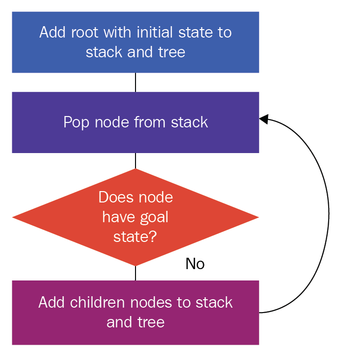
The steps in the preceding flowchart are as follows:

1. We create a root node using the initial state, and we add this to our stack and tree
2. We pop a node from the stack
3. We check whether it has the goal state; if it has the goal state, we stop our search here
4. If the answer to the condition in step 3 is No, then we find the child nodes of the pop node, and add them to the tree and stack
5. We repeat steps 2 to 4 until we either find the goal state or exhaust all of the nodes in the search tree

Let's apply the preceding algorithm to our filesystem, as follows:

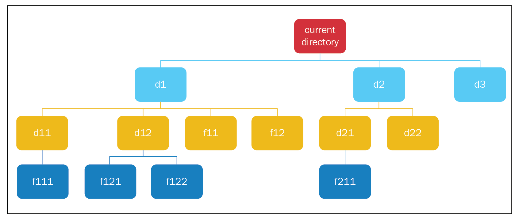
1. We create our root node, add it to the search tree, and add it to the stack. We pop a node from the stack, which is the current directory node.
2. The current directory node doesn't have the goal state, so we find its child nodes and add them to the tree and stack.

3. We pop a node from the stack (d1); it doesn't have the goal state, so we find its child nodes and add it to the tree and stack.
4. We pop a node from the stack (d11); it doesn't have the goal state, so we find its child node, add it to the tree and stack.
5. We pop a node (f111); it doesn't have the goal state, and it also doesn't have child nodes, so we carry on.
6. We pop the next node, d12; we find its child nodes and add them to the tree and stack.
7. We pop the next node, f121, and it doesn't have any child nodes, so we carry on.
8. We pop the next node, f122, and it doesn't have any child nodes, so we carry on.
9. We pop the next node, f11, and we encounter the same case (where we have no child nodes), so we carry on; the same goes for f12.
10. We pop the next node, d2, and we find its child nodes and add them to the tree and stack.
11. We pop the next node, d21, and we find its child node and add it to the tree and stack.
12. We pop the next node, f211, and we find that it has the goal state, so we end our search here.

Let's try to implement these steps in code, as follows:

...
from Node import Node
from State import State


def performStackDFS():
    """
    This function performs DFS search using a stack
    """
    #create stack
    stack = []
    
    #create root node and add to stack 
    initialState = State()
    root = Node(initialState)
    stack.append(root)
...

We have created a Python module called StackDFS.py, and it has a method called performStackDFS(). In this method, we have created an empty stack, which will hold all of our nodes, the initialState, a root node containing the initialState, and finally we have added this root node to the stack.

Remember that in Stack.py, we wrote a while loop to process all of the items in the stack. So, in the same way, in this case we will write a while loop to process all of the nodes in the stack:

...
while len(stack) > 0:
        
        #pop top node
        currentNode = stack.pop()
        
        print "-- pop --", currentNode.state.path
        
        #check if this is goal state
        if currentNode.state.checkGoalState():
            print "reached goal state"
            break
            
        #get the child nodes 
        childStates = currentNode.state.successorFunction()
        for childState in childStates:
            childNode = Node(State(childState))
            currentNode.addChild(childNode)

...

As shown in the preceding code, we pop the node from the top of the stack and call it currentNode(), and then we print it so that we can see the order in which the nodes are processed. We check whether the current node has the goal state, and if it does, we end our execution here. If it doesn't have the goal state, we find its child nodes and add it under currentNode, just like we did in NodeTest.py.

We will also add these child nodes to the stack, but in reverse order, using the following for loop:

...
for index in range(len(currentNode.children) - 1, -1, -1):
            stack.append(currentNode.children[index])

#print tree
    print "----------------------"
    root.printTree()
...

Finally, when we exit the while loop, we print the tree. Upon successful execution of the code, we will get the following output:

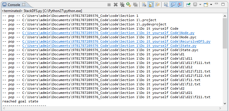
The output displays the order in which the nodes are processed, and we can see the first node of the tree. Finally, we encounter our goal state, and our search stops:

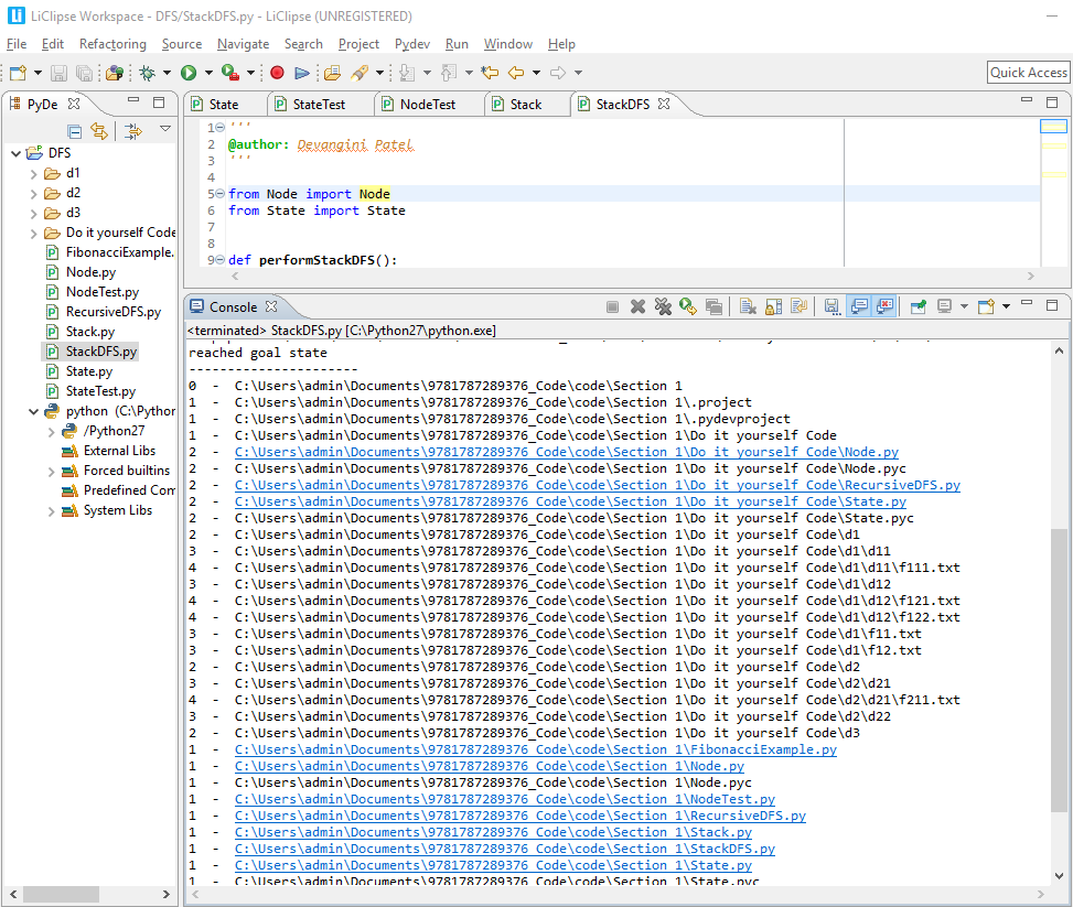
The preceding screenshot displays the search tree. Note that the preceding output and the one before it are almost the same. The only difference is that in the preceding screenshot, we can find two nodes, d22 and d3, because their parent nodes were explored.

When a function calls itself, we say that the function is a recursive function. Let's look at the example of the Fibonacci series. It is defined as follows: f(1) is equal to 1, f(2) is equal to 1, and for n greater than 2, f(n) is equal to f(n-1) + f(n-2). Let's look at the implementation of this function in code, as follows:

...
def fibonacci(n):
    if n <= 2:
        return 1
    else:
        return fibonacci(n-1) + fibonacci(n-2)

print "fibonacci(5)", fibonacci(5)
...

In the preceding code, we have created our function, fibonacci, which takes a number, n, as input. If n is less than or equal to 2, it returns 1; otherwise, it returns fibonacci(n-1) + fibonacci(n-2). Toward the end of the code, we have calculated the value of fibonacci(5), which is 5.

The output of running the preceding code is shown in the following screenshot:

If we want to visualize the recursion tree of the fibonacci function, we can go to https://visualgo.net/en/recursion. This website has visualizations of various data structures and algorithms.

The visualization of a recursion tree is as follows:

As shown in the preceding screenshot, the output that we get here is the same as the output we got with the code, and the order in which the nodes were explored is similar to DFS.

So, what happens when function 1 calls function 2? The program adds a stack frame to the program stack. A stack frame contains the local variables in function 1, the arguments passed to function 1, and the return addresses of function 2 and function 1.

Let's look at the example of the Fibonacci sequence again:

As you can see, the Fibonacci code has been modified for the sake of clarity. Suppose that the program is executing the line in bold, val2 = fibonacci(n-2). Then, the stack frame created will contain the following values—local variables is equal to val1, arguments passed is equal to n, and return address is the address of the code in bold.

This means that the return address points to the unprocessed curve. Because in recursion the program stack keeps a stack of unprocessed calls, instead of storing nodes in the stack, we will call DFS recursively on the child nodes, so that the stack is indirectly maintained.

Let's look at the steps of recursive DFS in the following diagram:

The steps in the preceding diagram are explained as follows:

1. We create an initial state.
2. We create a root node with this initial state.
3. We add the root node to the search tree and call DFS on the root node.
4. Recursive DFS is defined as follows: check whether the node has a goal state. If yes, then it returns the path; if no, then DFS finds the children node, and for each child node DFS adds the node to the tree, finally calling itself on the child node.

Now, we will apply the preceding algorithm to our filesystem, the steps for which are as follows:

1. We create the root node and add it to the search tree, and we call DFS on this root node.
2. When we call DFS on this root node, the function checks whether this node has the goal state, and it doesn't, so it finds its children nodes (d1, d2, and d3). It takes the first node, d1, adds it to the search tree, and calls DFS on the node.
3. When it calls DFS on d1, the function creates a program. When DFS is called on d1, then the program creates a stack frame and adds it to the program stack. In this case, we'll show the remaining nodes to be processed in the for loop. Here, we're adding d2 and d3 in the program stack.

4. When DFS is called on d1, it finds the children nodes d11, d12, f11, and f12, and adds d11 to the search tree.
5. It calls DFS on d11, and when it does so, it creates an entry in the program stack with the unprocessed nodes. Now, when DFS is called on d11, it finds the child node f111, adds f111 to the search tree, and calls DFS on the node.

6. When DFS is called on f111, it has no children nodes, so it returns back; when this happens, the program stack is unwounded, which means that the program returns execution and processes the last unprocessed nodes in the stack. In this case, it starts processing node d12. So, the program adds node d12 to the search tree, and calls DFS on d1.
7. When DFS is called on d12, it finds the children nodes f121 and f122. It adds node f121 to the search tree, and calls DFS on it. When DFS is called on f121, it adds the unprocessed node f122 to the stack.
8. When DFS is called on f121, it has no children nodes, so again the stack is unwounded. So, we process node f122. This node is added to the search tree and DFS is called on it. So, we continue processing the last node, f11, add it to the search tree, and call DFS on it.
9. When we call DFS on f11, it has no children nodes, so again the stack is unwounded. We continue processing node f12, it is added to the search tree, and DFS is called on f12. We encounter this case, and we continue processing node d2. We add it to the search tree, and we call DFS on d2.
10. When we call DFS on d2, we find that is has children nodes: d21 and d22. We add d21 to the search tree, and we call DFS on d21; when we call DFS on d21, it creates an entry for d22. In the program stack, when DFS is called on d21, we find that it has a child, f211. This node is added to the search tree and DFS is called on f211.
11. When DFS is called an f211, we realize that it has the goal state, and we end our search process here.

Let's look at how we can implement recursive DFS, as follows:

...
from State import State
from Node import Node


class RecursiveDFS():
    """
    This performs DFS search
    """
    def __init__(self):
        self.found = False
...

As shown in the preceding code, we have created a Python module called RecursiveDFS.py. It has a class called RecursiveDFS, and, in the constructor, it has a property called found, which indicates whether the solution has been found. We'll look at the significance of the found variable later.

Let's look at the following lines of code:

...
    def search(self):
        """
        This method performs the search
        """
        #get the initial state
        initialState = State()
        
        #create root node
        rootNode = Node(initialState)
        
        #perform search from root node
        self.DFS(rootNode)
        
        rootNode.printTree()
...

Here, we have a method called search, in which we are creating the initialState, and the rootNode we're calling the DFS function on the rootNode. Finally, we print the tree after we perform the DFS search, as follows:

...
def DFS(self, node):
        """
        This creates the search tree
        """
        if not self.found:
            print "-- proc --", node.state.path
            
            #check if we have reached goal state
            if node.state.checkGoalState():
                print "reached goal state"
                #self.found = True
                
            else:
                #find the successor states from current state 
                childStates = node.state.successorFunction()
                
                #add these states as children nodes of current node
                for childState in childStates:
                    childNode = Node(State(childState))
                    node.addChild(childNode)
                    
                    self.DFS(childNode)
....

The DFS function can be defined as follows:

• If the solution has not been found, then the node that is being processed is printed
• We check whether the node has the goal state, and if it does, we print that the goal state has been reached
• If it doesn't have the goal state, we find the child states; next, we create the child node for each child state, we add them to the tree, and we call DFS on each of the child nodes

Let's execute the program; we will get the following output:

When we processed f211, we reached the goal state, but here we have three extra lines; this is because these nodes have been added to the program stack. To remove these lines, we have created a variable called found, so that when the goal state is found, the variable will be set to True. Once we encounter f211, the remaining nodes in the program stack will not be processed:

Let's run this code again and see what happens:

As you can see, once we've processed f211 and reached the goal state, the node processing stops. The output of the printTree function is the same as what we store in StackDFS.py.

Now that you understand how DFS can be made into a recursive function, in the next topic we will look at an application that you can develop by yourself.